視覺化工具

注意

在 Colab 上嘗試 或 跳轉至末尾 下載完整示例程式碼。

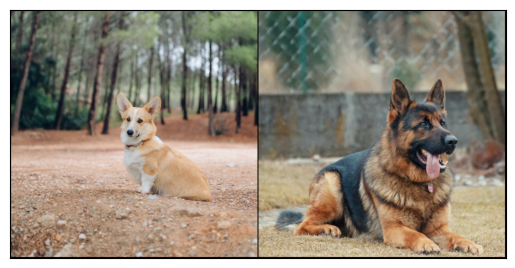
此示例演示了 torchvision 提供的一些用於視覺化影像、邊界框、分割掩碼和關鍵點的工具函式。

import torch
import numpy as np
import matplotlib.pyplot as plt

import torchvision.transforms.functional as F


plt.rcParams["savefig.bbox"] = 'tight'


def show(imgs):
    if not isinstance(imgs, list):
        imgs = [imgs]
    fig, axs = plt.subplots(ncols=len(imgs), squeeze=False)
    for i, img in enumerate(imgs):
        img = img.detach()
        img = F.to_pil_image(img)
        axs[0, i].imshow(np.asarray(img))
        axs[0, i].set(xticklabels=[], yticklabels=[], xticks=[], yticks=[])

視覺化影像網格

函式 make_grid() 可用於建立表示多個影像網格的張量。此工具函式需要一個 dtype 為 uint8 的單張影像作為輸入。

from torchvision.utils import make_grid
from torchvision.io import decode_image
from pathlib import Path

dog1_int = decode_image(str(Path('../assets') / 'dog1.jpg'))
dog2_int = decode_image(str(Path('../assets') / 'dog2.jpg'))
dog_list = [dog1_int, dog2_int]

grid = make_grid(dog_list)
show(grid)

視覺化邊界框

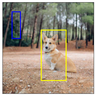
我們可以使用 draw_bounding_boxes() 在影像上繪製框。我們可以設定顏色、標籤、寬度以及字型和字型大小。框的格式為 (xmin, ymin, xmax, ymax)。

from torchvision.utils import draw_bounding_boxes


boxes = torch.tensor([[50, 50, 100, 200], [210, 150, 350, 430]], dtype=torch.float)
colors = ["blue", "yellow"]
result = draw_bounding_boxes(dog1_int, boxes, colors=colors, width=5)
show(result)

自然地，我們也可以繪製 torchvision 檢測模型產生的邊界框。這裡是一個使用從 fasterrcnn_resnet50_fpn() 模型載入的 Faster R-CNN 模型的演示。有關此類模型輸出的更多詳細資訊，您可以參考 例項分割模型。

from torchvision.models.detection import fasterrcnn_resnet50_fpn, FasterRCNN_ResNet50_FPN_Weights


weights = FasterRCNN_ResNet50_FPN_Weights.DEFAULT
transforms = weights.transforms()

images = [transforms(d) for d in dog_list]

model = fasterrcnn_resnet50_fpn(weights=weights, progress=False)
model = model.eval()

outputs = model(images)
print(outputs)

[{'boxes': tensor([[215.9767, 171.1661, 402.0078, 378.7391],
        [344.6341, 172.6735, 357.6114, 220.1435],
        [153.1306, 185.5567, 172.9223, 254.7014]], grad_fn=<StackBackward0>), 'labels': tensor([18,  1,  1]), 'scores': tensor([0.9989, 0.0701, 0.0611], grad_fn=<IndexBackward0>)}, {'boxes': tensor([[ 23.5964, 132.4331, 449.9359, 493.0222],
        [225.8182, 124.6292, 467.2861, 492.2621],
        [ 18.5248, 135.4171, 420.9786, 479.2225]], grad_fn=<StackBackward0>), 'labels': tensor([18, 18, 17]), 'scores': tensor([0.9980, 0.0879, 0.0671], grad_fn=<IndexBackward0>)}]

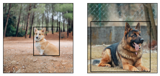
讓我們繪製模型檢測到的框。我們只會繪製分數高於給定閾值的框。

score_threshold = .8
dogs_with_boxes = [
    draw_bounding_boxes(dog_int, boxes=output['boxes'][output['scores'] > score_threshold], width=4)
    for dog_int, output in zip(dog_list, outputs)
]
show(dogs_with_boxes)

視覺化分割掩碼

函式 draw_segmentation_masks() 可用於在影像上繪製分割掩碼。語義分割模型和例項分割模型的輸出不同，因此我們將分別處理它們。

語義分割模型

我們將看到如何將其與使用 fcn_resnet50() 載入的 torchvision 的 FCN Resnet-50 一起使用。首先讓我們看一下模型的輸出。

from torchvision.models.segmentation import fcn_resnet50, FCN_ResNet50_Weights

weights = FCN_ResNet50_Weights.DEFAULT
transforms = weights.transforms(resize_size=None)

model = fcn_resnet50(weights=weights, progress=False)
model = model.eval()

batch = torch.stack([transforms(d) for d in dog_list])
output = model(batch)['out']
print(output.shape, output.min().item(), output.max().item())

Downloading: "https://download.pytorch.org/models/fcn_resnet50_coco-1167a1af.pth" to /root/.cache/torch/hub/checkpoints/fcn_resnet50_coco-1167a1af.pth
torch.Size([2, 21, 500, 500]) -7.089669704437256 14.858257293701172

如上所示，分割模型的輸出是形狀為 (batch_size, num_classes, H, W) 的張量。每個值都是一個未歸一化的分數，我們可以透過使用 softmax 將它們歸一化到 [0, 1]。在 softmax 之後，我們可以將每個值解釋為一個機率，表示給定畫素屬於給定類別的可能性有多大。

讓我們繪製檢測到的狗類別和船類別的掩碼

sem_class_to_idx = {cls: idx for (idx, cls) in enumerate(weights.meta["categories"])}

normalized_masks = torch.nn.functional.softmax(output, dim=1)

dog_and_boat_masks = [
    normalized_masks[img_idx, sem_class_to_idx[cls]]
    for img_idx in range(len(dog_list))
    for cls in ('dog', 'boat')
]

show(dog_and_boat_masks)

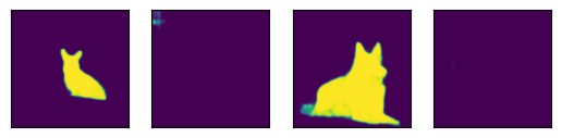
正如預期的那樣，模型對狗類別很自信，但對船類別則不太自信。

函式 draw_segmentation_masks() 可用於在原始影像上方繪製這些掩碼。此函式期望掩碼是布林掩碼，但我們上面的掩碼包含 [0, 1] 範圍內的機率。要獲得布林掩碼，我們可以執行以下操作

class_dim = 1
boolean_dog_masks = (normalized_masks.argmax(class_dim) == sem_class_to_idx['dog'])
print(f"shape = {boolean_dog_masks.shape}, dtype = {boolean_dog_masks.dtype}")
show([m.float() for m in boolean_dog_masks])

shape = torch.Size([2, 500, 500]), dtype = torch.bool

上面定義 boolean_dog_masks 的那行程式碼有點晦澀難懂，但您可以將其理解為以下查詢：“哪些畫素最有可能屬於‘狗’類別？”

注意

雖然我們在這裡使用了 normalized_masks，但直接使用模型的未歸一化分數也會得到相同的結果（因為 softmax 操作保留了順序）。

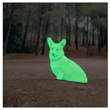
現在我們有了布林掩碼，可以將它們與 draw_segmentation_masks() 一起使用，在原始影像上方繪製它們

from torchvision.utils import draw_segmentation_masks

dogs_with_masks = [
    draw_segmentation_masks(img, masks=mask, alpha=0.7)
    for img, mask in zip(dog_list, boolean_dog_masks)
]
show(dogs_with_masks)

我們可以為每張影像繪製多個掩碼！記住，模型返回的掩碼數量與類別數量相同。讓我們提出與上面相同的查詢，但這次是針對所有類別，而不僅僅是狗類別：“對於每個畫素和每個類別 C，類別 C 是最有可能的類別嗎？”

這個過程有點複雜，所以我們首先演示如何處理單張影像，然後再推廣到整個批次。

num_classes = normalized_masks.shape[1]
dog1_masks = normalized_masks[0]
class_dim = 0
dog1_all_classes_masks = dog1_masks.argmax(class_dim) == torch.arange(num_classes)[:, None, None]

print(f"dog1_masks shape = {dog1_masks.shape}, dtype = {dog1_masks.dtype}")
print(f"dog1_all_classes_masks = {dog1_all_classes_masks.shape}, dtype = {dog1_all_classes_masks.dtype}")

dog_with_all_masks = draw_segmentation_masks(dog1_int, masks=dog1_all_classes_masks, alpha=.6)
show(dog_with_all_masks)

dog1_masks shape = torch.Size([21, 500, 500]), dtype = torch.float32
dog1_all_classes_masks = torch.Size([21, 500, 500]), dtype = torch.bool

從上面的影像中我們可以看到，只繪製了 2 個掩碼：背景的掩碼和狗的掩碼。這是因為模型認為在所有畫素中，只有這兩個類別是最有可能的。如果模型在其他畫素中檢測到另一個類別是最有可能的，我們就會在上面看到它的掩碼。

移除背景掩碼很簡單，只需傳遞 masks=dog1_all_classes_masks[1:] 即可，因為背景類別是索引為 0 的類別。

現在讓我們對整個影像批次做同樣的處理。程式碼類似，但涉及更多關於維度的操作。

class_dim = 1
all_classes_masks = normalized_masks.argmax(class_dim) == torch.arange(num_classes)[:, None, None, None]
print(f"shape = {all_classes_masks.shape}, dtype = {all_classes_masks.dtype}")
# The first dimension is the classes now, so we need to swap it
all_classes_masks = all_classes_masks.swapaxes(0, 1)

dogs_with_masks = [
    draw_segmentation_masks(img, masks=mask, alpha=.6)
    for img, mask in zip(dog_list, all_classes_masks)
]
show(dogs_with_masks)

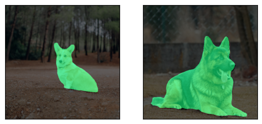
shape = torch.Size([21, 2, 500, 500]), dtype = torch.bool

例項分割模型

例項分割模型與語義分割模型的輸出顯著不同。我們將在這裡看到如何繪製這類模型的掩碼。首先讓我們分析 Mask-RCNN 模型的輸出。請注意，這些模型不需要影像歸一化，因此我們不需要使用歸一化的批次。

注意

我們將在這裡描述 Mask-RCNN 模型的輸出。目標檢測、例項分割和人體關鍵點檢測 中的模型都具有相似的輸出格式，但其中一些可能包含額外資訊，例如 keypointrcnn_resnet50_fpn() 的關鍵點，而有些可能不包含掩碼，例如 fasterrcnn_resnet50_fpn()。

from torchvision.models.detection import maskrcnn_resnet50_fpn, MaskRCNN_ResNet50_FPN_Weights

weights = MaskRCNN_ResNet50_FPN_Weights.DEFAULT
transforms = weights.transforms()

images = [transforms(d) for d in dog_list]

model = maskrcnn_resnet50_fpn(weights=weights, progress=False)
model = model.eval()

output = model(images)
print(output)

Downloading: "https://download.pytorch.org/models/maskrcnn_resnet50_fpn_coco-bf2d0c1e.pth" to /root/.cache/torch/hub/checkpoints/maskrcnn_resnet50_fpn_coco-bf2d0c1e.pth
[{'boxes': tensor([[219.7444, 168.1722, 400.7378, 384.0263],
        [343.9716, 171.2287, 358.3447, 222.6263],
        [301.0303, 192.6917, 313.8879, 232.3154]], grad_fn=<StackBackward0>), 'labels': tensor([18,  1,  1]), 'scores': tensor([0.9987, 0.7187, 0.6525], grad_fn=<IndexBackward0>), 'masks': tensor([[[[0., 0., 0.,  ..., 0., 0., 0.],
          [0., 0., 0.,  ..., 0., 0., 0.],
          [0., 0., 0.,  ..., 0., 0., 0.],
          ...,
          [0., 0., 0.,  ..., 0., 0., 0.],
          [0., 0., 0.,  ..., 0., 0., 0.],
          [0., 0., 0.,  ..., 0., 0., 0.]]],


        [[[0., 0., 0.,  ..., 0., 0., 0.],
          [0., 0., 0.,  ..., 0., 0., 0.],
          [0., 0., 0.,  ..., 0., 0., 0.],
          ...,
          [0., 0., 0.,  ..., 0., 0., 0.],
          [0., 0., 0.,  ..., 0., 0., 0.],
          [0., 0., 0.,  ..., 0., 0., 0.]]],


        [[[0., 0., 0.,  ..., 0., 0., 0.],
          [0., 0., 0.,  ..., 0., 0., 0.],
          [0., 0., 0.,  ..., 0., 0., 0.],
          ...,
          [0., 0., 0.,  ..., 0., 0., 0.],
          [0., 0., 0.,  ..., 0., 0., 0.],
          [0., 0., 0.,  ..., 0., 0., 0.]]]], grad_fn=<UnsqueezeBackward0>)}, {'boxes': tensor([[ 44.6767, 137.9018, 446.5324, 487.3429],
        [  0.0000, 288.0053, 489.9292, 490.2352]], grad_fn=<StackBackward0>), 'labels': tensor([18, 15]), 'scores': tensor([0.9978, 0.0697], grad_fn=<IndexBackward0>), 'masks': tensor([[[[0., 0., 0.,  ..., 0., 0., 0.],
          [0., 0., 0.,  ..., 0., 0., 0.],
          [0., 0., 0.,  ..., 0., 0., 0.],
          ...,
          [0., 0., 0.,  ..., 0., 0., 0.],
          [0., 0., 0.,  ..., 0., 0., 0.],
          [0., 0., 0.,  ..., 0., 0., 0.]]],


        [[[0., 0., 0.,  ..., 0., 0., 0.],
          [0., 0., 0.,  ..., 0., 0., 0.],
          [0., 0., 0.,  ..., 0., 0., 0.],
          ...,
          [0., 0., 0.,  ..., 0., 0., 0.],
          [0., 0., 0.,  ..., 0., 0., 0.],
          [0., 0., 0.,  ..., 0., 0., 0.]]]], grad_fn=<UnsqueezeBackward0>)}]

讓我們分解一下。對於批次中的每張影像，模型會輸出一些檢測結果（或例項）。每張輸入影像的檢測數量各不相同。每個例項都由其邊界框、標籤、分數和掩碼描述。

輸出的組織方式如下：輸出是一個長度為 batch_size 的列表。列表中的每個條目對應一張輸入影像，它是一個字典，包含鍵‘boxes’、‘labels’、‘scores’和‘masks’。與這些鍵關聯的每個值都包含 num_instances 個元素。在上面的例子中，第一張影像檢測到 3 個例項，第二張檢測到 2 個例項。

如上所述，可以使用 draw_bounding_boxes() 繪製邊界框，但在這裡我們更關注掩碼。這些掩碼與我們在上面看到的語義分割模型的掩碼截然不同。

dog1_output = output[0]
dog1_masks = dog1_output['masks']
print(f"shape = {dog1_masks.shape}, dtype = {dog1_masks.dtype}, "
      f"min = {dog1_masks.min()}, max = {dog1_masks.max()}")

shape = torch.Size([3, 1, 500, 500]), dtype = torch.float32, min = 0.0, max = 0.9999862909317017

這裡的掩碼對應於機率，指示每個畫素屬於該例項預測標籤的可能性。這些預測標籤對應於同一輸出字典中的‘labels’元素。讓我們看看第一張影像的例項預測了哪些標籤。

print("For the first dog, the following instances were detected:")
print([weights.meta["categories"][label] for label in dog1_output['labels']])

For the first dog, the following instances were detected:
['dog', 'person', 'person']

有趣的是，模型在影像中檢測到兩個人。讓我們繼續繪製這些掩碼。draw_segmentation_masks() 函式需要布林掩碼，因此我們需要將這些機率轉換為布林值。記住，這些掩碼的語義是“此畫素屬於預測類別的可能性有多大？”。因此，將這些掩碼轉換為布林值的一個自然方法是使用 0.5 的機率進行閾值處理（也可以選擇不同的閾值）。

proba_threshold = 0.5
dog1_bool_masks = dog1_output['masks'] > proba_threshold
print(f"shape = {dog1_bool_masks.shape}, dtype = {dog1_bool_masks.dtype}")

# There's an extra dimension (1) to the masks. We need to remove it
dog1_bool_masks = dog1_bool_masks.squeeze(1)

show(draw_segmentation_masks(dog1_int, dog1_bool_masks, alpha=0.9))

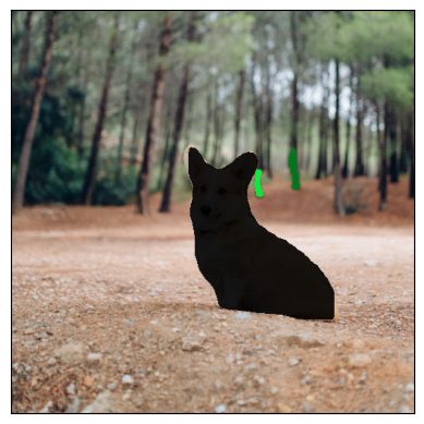
shape = torch.Size([3, 1, 500, 500]), dtype = torch.bool

模型似乎正確地檢測到了狗，但也將樹木誤認為是人。更仔細地檢視分數將有助於我們繪製更相關的掩碼。

print(dog1_output['scores'])

tensor([0.9987, 0.7187, 0.6525], grad_fn=<IndexBackward0>)

顯然，模型對狗的檢測比對人的檢測更有信心。這是個好訊息。在繪製掩碼時，我們可以只選擇得分較高的掩碼。這裡我們使用 0.75 的分數閾值，並繪製第二隻狗的掩碼。

score_threshold = .75

boolean_masks = [
    out['masks'][out['scores'] > score_threshold] > proba_threshold
    for out in output
]

dogs_with_masks = [
    draw_segmentation_masks(img, mask.squeeze(1))
    for img, mask in zip(dog_list, boolean_masks)
]
show(dogs_with_masks)

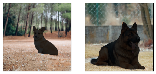
第一張影像中的兩個‘人’的掩碼未被選中，因為它們的得分低於分數閾值。類似地，在第二張影像中，類別為 15（對應‘長凳’）的例項也未被選中。

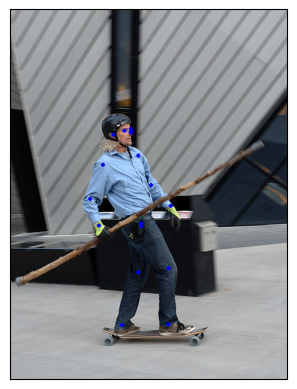
視覺化關鍵點

函式 draw_keypoints() 可用於在影像上繪製關鍵點。我們將看到如何將其與使用 keypointrcnn_resnet50_fpn() 載入的 torchvision 的 KeypointRCNN 一起使用。我們首先將檢視模型的輸出。

from torchvision.models.detection import keypointrcnn_resnet50_fpn, KeypointRCNN_ResNet50_FPN_Weights
from torchvision.io import decode_image

person_int = decode_image(str(Path("../assets") / "person1.jpg"))

weights = KeypointRCNN_ResNet50_FPN_Weights.DEFAULT
transforms = weights.transforms()

person_float = transforms(person_int)

model = keypointrcnn_resnet50_fpn(weights=weights, progress=False)
model = model.eval()

outputs = model([person_float])
print(outputs)

Downloading: "https://download.pytorch.org/models/keypointrcnn_resnet50_fpn_coco-fc266e95.pth" to /root/.cache/torch/hub/checkpoints/keypointrcnn_resnet50_fpn_coco-fc266e95.pth
[{'boxes': tensor([[124.3751, 177.9242, 327.6354, 574.7064],
        [124.3625, 180.7574, 290.1061, 390.7958]], grad_fn=<StackBackward0>), 'labels': tensor([1, 1]), 'scores': tensor([0.9998, 0.1070], grad_fn=<IndexBackward0>), 'keypoints': tensor([[[208.0176, 214.2408,   1.0000],
         [208.0176, 207.0375,   1.0000],
         [197.8246, 210.6392,   1.0000],
         [208.0176, 211.8398,   1.0000],
         [178.6378, 217.8425,   1.0000],
         [221.2086, 253.8590,   1.0000],
         [160.6502, 269.4662,   1.0000],
         [243.9929, 304.2822,   1.0000],
         [138.4654, 328.8935,   1.0000],
         [277.5698, 340.8990,   1.0000],
         [153.4551, 374.5144,   1.0000],
         [226.0053, 375.7150,   1.0000],
         [226.0053, 370.3125,   1.0000],
         [221.8082, 455.5516,   1.0000],
         [273.9723, 448.9486,   1.0000],
         [193.6275, 546.1932,   1.0000],
         [273.3727, 545.5930,   1.0000]],

        [[207.8327, 214.6636,   1.0000],
         [207.2343, 207.4622,   1.0000],
         [198.2590, 209.8627,   1.0000],
         [208.4310, 210.4628,   1.0000],
         [178.5134, 218.2642,   1.0000],
         [219.7997, 251.8704,   1.0000],
         [162.3579, 269.2736,   1.0000],
         [245.5289, 304.6800,   1.0000],
         [138.4238, 330.4848,   1.0000],
         [278.4382, 346.0876,   1.0000],
         [153.3826, 374.8929,   1.0000],
         [233.5618, 368.2917,   1.0000],
         [225.7832, 367.6916,   1.0000],
         [289.8069, 357.4897,   1.0000],
         [245.5289, 389.8956,   1.0000],
         [281.4300, 349.0882,   1.0000],
         [209.0294, 389.8956,   1.0000]]], grad_fn=<CopySlices>), 'keypoints_scores': tensor([[16.0163, 16.6672, 15.8312,  4.6510, 14.2053,  8.8280,  9.1136, 12.2084,
         12.1901, 13.8453, 10.7090,  5.5852,  7.5005, 11.3378,  9.3700,  8.2987,
          8.4479],
        [12.9326, 13.8158, 14.9053,  3.9368, 12.9585,  6.4240,  6.8328, 10.4227,
          9.2907, 10.1066, 10.1019,  0.1822,  4.3057, -4.9904, -2.7409, -2.7874,
         -3.9329]], grad_fn=<CopySlices>)}]

如我們所見，輸出包含一個字典列表。輸出列表的長度為 batch_size。我們目前只有一張影像，因此列表長度為 1。列表中的每個條目對應一張輸入影像，它是一個字典，包含鍵 boxes、labels、scores、keypoints 和 keypoint_scores。與這些鍵關聯的每個值都包含 num_instances 個元素。在上面的例子中，影像中檢測到 2 個例項。

kpts = outputs[0]['keypoints']
scores = outputs[0]['scores']

print(kpts)
print(scores)

tensor([[[208.0176, 214.2408,   1.0000],
         [208.0176, 207.0375,   1.0000],
         [197.8246, 210.6392,   1.0000],
         [208.0176, 211.8398,   1.0000],
         [178.6378, 217.8425,   1.0000],
         [221.2086, 253.8590,   1.0000],
         [160.6502, 269.4662,   1.0000],
         [243.9929, 304.2822,   1.0000],
         [138.4654, 328.8935,   1.0000],
         [277.5698, 340.8990,   1.0000],
         [153.4551, 374.5144,   1.0000],
         [226.0053, 375.7150,   1.0000],
         [226.0053, 370.3125,   1.0000],
         [221.8082, 455.5516,   1.0000],
         [273.9723, 448.9486,   1.0000],
         [193.6275, 546.1932,   1.0000],
         [273.3727, 545.5930,   1.0000]],

        [[207.8327, 214.6636,   1.0000],
         [207.2343, 207.4622,   1.0000],
         [198.2590, 209.8627,   1.0000],
         [208.4310, 210.4628,   1.0000],
         [178.5134, 218.2642,   1.0000],
         [219.7997, 251.8704,   1.0000],
         [162.3579, 269.2736,   1.0000],
         [245.5289, 304.6800,   1.0000],
         [138.4238, 330.4848,   1.0000],
         [278.4382, 346.0876,   1.0000],
         [153.3826, 374.8929,   1.0000],
         [233.5618, 368.2917,   1.0000],
         [225.7832, 367.6916,   1.0000],
         [289.8069, 357.4897,   1.0000],
         [245.5289, 389.8956,   1.0000],
         [281.4300, 349.0882,   1.0000],
         [209.0294, 389.8956,   1.0000]]], grad_fn=<CopySlices>)
tensor([0.9998, 0.1070], grad_fn=<IndexBackward0>)

KeypointRCNN 模型檢測到影像中有兩個例項。如果使用 draw_bounding_boxes() 繪製邊界框，您會認出它們是人和衝浪板。如果我們檢視分數，就會發現模型對人的檢測比對沖浪板的檢測更有信心。現在我們可以設定一個置信度閾值，並繪製我們足夠自信的例項。讓我們設定一個 0.75 的閾值，並過濾出對應於人的關鍵點。

detect_threshold = 0.75
idx = torch.where(scores > detect_threshold)
keypoints = kpts[idx]

print(keypoints)

tensor([[[208.0176, 214.2408,   1.0000],
         [208.0176, 207.0375,   1.0000],
         [197.8246, 210.6392,   1.0000],
         [208.0176, 211.8398,   1.0000],
         [178.6378, 217.8425,   1.0000],
         [221.2086, 253.8590,   1.0000],
         [160.6502, 269.4662,   1.0000],
         [243.9929, 304.2822,   1.0000],
         [138.4654, 328.8935,   1.0000],
         [277.5698, 340.8990,   1.0000],
         [153.4551, 374.5144,   1.0000],
         [226.0053, 375.7150,   1.0000],
         [226.0053, 370.3125,   1.0000],
         [221.8082, 455.5516,   1.0000],
         [273.9723, 448.9486,   1.0000],
         [193.6275, 546.1932,   1.0000],
         [273.3727, 545.5930,   1.0000]]], grad_fn=<IndexBackward0>)

太好了，現在我們有了對應於人的關鍵點。每個關鍵點由 x, y 座標和可見性表示。現在我們可以使用 draw_keypoints() 函式繪製關鍵點。注意，該工具函式需要 uint8 影像。

from torchvision.utils import draw_keypoints

res = draw_keypoints(person_int, keypoints, colors="blue", radius=3)
show(res)

正如我們所見，關鍵點在影像上方顯示為彩色圓圈。一個人的 coco 關鍵點是有序的，表示以下列表。

coco_keypoints = [
    "nose", "left_eye", "right_eye", "left_ear", "right_ear",
    "left_shoulder", "right_shoulder", "left_elbow", "right_elbow",
    "left_wrist", "right_wrist", "left_hip", "right_hip",
    "left_knee", "right_knee", "left_ankle", "right_ankle",
]

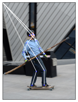
如果我們有興趣連線關鍵點怎麼辦？這在建立姿態檢測或行為識別時特別有用。我們可以使用 connectivity 引數輕鬆連線關鍵點。仔細觀察會發現，我們需要按以下順序連線點以構建人體骨骼。

鼻子 -> 左眼 -> 左耳。(0, 1), (1, 3)

鼻子 -> 右眼 -> 右耳。(0, 2), (2, 4)

鼻子 -> 左肩 -> 左肘 -> 左腕。(0, 5), (5, 7), (7, 9)

鼻子 -> 右肩 -> 右肘 -> 右腕。(0, 6), (6, 8), (8, 10)

左肩 -> 左臀 -> 左膝 -> 左踝。(5, 11), (11, 13), (13, 15)

右肩 -> 右臀 -> 右膝 -> 右踝。(6, 12), (12, 14), (14, 16)

我們將建立一個包含這些要連線的關鍵點 ID 的列表。

connect_skeleton = [
    (0, 1), (0, 2), (1, 3), (2, 4), (0, 5), (0, 6), (5, 7), (6, 8),
    (7, 9), (8, 10), (5, 11), (6, 12), (11, 13), (12, 14), (13, 15), (14, 16)
]

我們將上面的列表傳遞給 connectivity 引數來連線關鍵點。

res = draw_keypoints(person_int, keypoints, connectivity=connect_skeleton, colors="blue", radius=4, width=3)
show(res)

看起來相當不錯。

繪製帶有可見性的關鍵點

讓我們看看另一個關鍵點預測模組產生的結果，並顯示連線性

prediction = torch.tensor(
    [[[208.0176, 214.2409, 1.0000],
      [000.0000, 000.0000, 0.0000],
      [197.8246, 210.6392, 1.0000],
      [000.0000, 000.0000, 0.0000],
      [178.6378, 217.8425, 1.0000],
      [221.2086, 253.8591, 1.0000],
      [160.6502, 269.4662, 1.0000],
      [243.9929, 304.2822, 1.0000],
      [138.4654, 328.8935, 1.0000],
      [277.5698, 340.8990, 1.0000],
      [153.4551, 374.5145, 1.0000],
      [000.0000, 000.0000, 0.0000],
      [226.0053, 370.3125, 1.0000],
      [221.8081, 455.5516, 1.0000],
      [273.9723, 448.9486, 1.0000],
      [193.6275, 546.1933, 1.0000],
      [273.3727, 545.5930, 1.0000]]]
)

res = draw_keypoints(person_int, prediction, connectivity=connect_skeleton, colors="blue", radius=4, width=3)
show(res)

那裡發生了什麼？預測新關鍵點的模型無法檢測到滑板運動員左上方身體上隱藏的三個點。更準確地說，模型預測左眼、左耳和左臀的關鍵點為 (x, y, vis) = (0, 0, 0)。所以我們肯定不想顯示這些關鍵點和連線，而且你也不必這樣做。檢視 draw_keypoints() 的引數，我們可以看到可以將一個可見性張量作為附加引數傳遞。根據模型的預測，可見性是關鍵點的第三個維度，我們只需將其提取出來即可。讓我們將 prediction 分割成關鍵點座標和它們各自的可見性，並將它們都作為引數傳遞給 draw_keypoints()。

coordinates, visibility = prediction.split([2, 1], dim=-1)
visibility = visibility.bool()

res = draw_keypoints(
    person_int, coordinates, visibility=visibility, connectivity=connect_skeleton, colors="blue", radius=4, width=3
)
show(res)

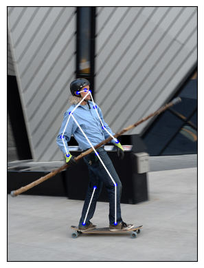
我們可以看到未檢測到的關鍵點沒有被繪製出來，並且跳過了不可見的關鍵點連線。這可以減少多重檢測影像上的噪聲，或者像我們這樣的情況，關鍵點預測模型遺漏了一些檢測。大多數 torch 關鍵點預測模型會返回每個預測的可見性，您可以直接使用。我們在第一個例子中使用的 keypointrcnn_resnet50_fpn() 模型也是如此。