計算機視覺遷移學習教程

建立日期: 2017 年 3 月 24 日 | 最後更新日期: 2025 年 1 月 27 日 | 最後驗證日期: 2024 年 11 月 05 日

作者: Sasank Chilamkurthy

在本教程中，你將學習如何使用遷移學習訓練一個用於影像分類的卷積神經網路。你可以在 cs231n 筆記中閱讀更多關於遷移學習的內容。

引用這些筆記：

實際上，很少有人會從頭開始訓練一個完整的卷積網路（使用隨機初始化），因為擁有足夠大的資料集的情況相對罕見。相反，常見的做法是在一個非常大的資料集（例如 ImageNet，包含 120 萬張影像和 1000 個類別）上預訓練一個 ConvNet，然後將該 ConvNet 用作目標任務的初始化或固定特徵提取器。

這兩種主要的遷移學習場景如下：

• 微調 ConvNet：不是使用隨機初始化，我們使用預訓練的網路（例如在 imagenet 1000 資料集上訓練的網路）初始化網路。其餘的訓練過程照常進行。

• 將 ConvNet 作為固定特徵提取器：在這裡，我們將凍結除了最終全連線層之外的所有網路權重。這個最後一個全連線層將被一個具有隨機權重的新層取代，並且只訓練這一層。

# License: BSD
# Author: Sasank Chilamkurthy

import torch
import torch.nn as nn
import torch.optim as optim
from torch.optim import lr_scheduler
import torch.backends.cudnn as cudnn
import numpy as np
import torchvision
from torchvision import datasets, models, transforms
import matplotlib.pyplot as plt
import time
import os
from PIL import Image
from tempfile import TemporaryDirectory

cudnn.benchmark = True
plt.ion()   # interactive mode

<contextlib.ExitStack object at 0x7f5645de7790>

載入資料

我們將使用 torchvision 和 torch.utils.data 包來載入資料。

我們今天將解決的問題是訓練一個模型來分類螞蟻和蜜蜂。我們有大約 120 張螞蟻和蜜蜂的訓練影像，每個類別各有約 120 張。每個類別有 75 張驗證影像。通常，如果從頭開始訓練，這是一個非常小的資料集，難以進行泛化。由於我們使用遷移學習，我們應該能夠相當好地泛化。

這個資料集是 imagenet 的一個非常小的子集。

注意

從此處下載資料並將其解壓到當前目錄。

# Data augmentation and normalization for training
# Just normalization for validation
data_transforms = {
    'train': transforms.Compose([
        transforms.RandomResizedCrop(224),
        transforms.RandomHorizontalFlip(),
        transforms.ToTensor(),
        transforms.Normalize([0.485, 0.456, 0.406], [0.229, 0.224, 0.225])
    ]),
    'val': transforms.Compose([
        transforms.Resize(256),
        transforms.CenterCrop(224),
        transforms.ToTensor(),
        transforms.Normalize([0.485, 0.456, 0.406], [0.229, 0.224, 0.225])
    ]),
}

data_dir = 'data/hymenoptera_data'
image_datasets = {x: datasets.ImageFolder(os.path.join(data_dir, x),
                                          data_transforms[x])
                  for x in ['train', 'val']}
dataloaders = {x: torch.utils.data.DataLoader(image_datasets[x], batch_size=4,
                                             shuffle=True, num_workers=4)
              for x in ['train', 'val']}
dataset_sizes = {x: len(image_datasets[x]) for x in ['train', 'val']}
class_names = image_datasets['train'].classes

# We want to be able to train our model on an `accelerator <https://pytorch.com.tw/docs/stable/torch.html#accelerators>`__
# such as CUDA, MPS, MTIA, or XPU. If the current accelerator is available, we will use it. Otherwise, we use the CPU.

device = torch.accelerator.current_accelerator().type if torch.accelerator.is_available() else "cpu"
print(f"Using {device} device")

Using cuda device

視覺化一些影像

讓我們視覺化一些訓練影像，以便理解資料增強。

def imshow(inp, title=None):
    """Display image for Tensor."""
    inp = inp.numpy().transpose((1, 2, 0))
    mean = np.array([0.485, 0.456, 0.406])
    std = np.array([0.229, 0.224, 0.225])
    inp = std * inp + mean
    inp = np.clip(inp, 0, 1)
    plt.imshow(inp)
    if title is not None:
        plt.title(title)
    plt.pause(0.001)  # pause a bit so that plots are updated


# Get a batch of training data
inputs, classes = next(iter(dataloaders['train']))

# Make a grid from batch
out = torchvision.utils.make_grid(inputs)

imshow(out, title=[class_names[x] for x in classes])

訓練模型

現在，讓我們編寫一個通用的函式來訓練模型。這裡我們將說明：

• 排程學習率

• 儲存最佳模型

在下文中，引數 scheduler 是來自 torch.optim.lr_scheduler 的學習率排程器物件。

def train_model(model, criterion, optimizer, scheduler, num_epochs=25):
    since = time.time()

    # Create a temporary directory to save training checkpoints
    with TemporaryDirectory() as tempdir:
        best_model_params_path = os.path.join(tempdir, 'best_model_params.pt')

        torch.save(model.state_dict(), best_model_params_path)
        best_acc = 0.0

        for epoch in range(num_epochs):
            print(f'Epoch {epoch}/{num_epochs - 1}')
            print('-' * 10)

            # Each epoch has a training and validation phase
            for phase in ['train', 'val']:
                if phase == 'train':
                    model.train()  # Set model to training mode
                else:
                    model.eval()   # Set model to evaluate mode

                running_loss = 0.0
                running_corrects = 0

                # Iterate over data.
                for inputs, labels in dataloaders[phase]:
                    inputs = inputs.to(device)
                    labels = labels.to(device)

                    # zero the parameter gradients
                    optimizer.zero_grad()

                    # forward
                    # track history if only in train
                    with torch.set_grad_enabled(phase == 'train'):
                        outputs = model(inputs)
                        _, preds = torch.max(outputs, 1)
                        loss = criterion(outputs, labels)

                        # backward + optimize only if in training phase
                        if phase == 'train':
                            loss.backward()
                            optimizer.step()

                    # statistics
                    running_loss += loss.item() * inputs.size(0)
                    running_corrects += torch.sum(preds == labels.data)
                if phase == 'train':
                    scheduler.step()

                epoch_loss = running_loss / dataset_sizes[phase]
                epoch_acc = running_corrects.double() / dataset_sizes[phase]

                print(f'{phase} Loss: {epoch_loss:.4f} Acc: {epoch_acc:.4f}')

                # deep copy the model
                if phase == 'val' and epoch_acc > best_acc:
                    best_acc = epoch_acc
                    torch.save(model.state_dict(), best_model_params_path)

            print()

        time_elapsed = time.time() - since
        print(f'Training complete in {time_elapsed // 60:.0f}m {time_elapsed % 60:.0f}s')
        print(f'Best val Acc: {best_acc:4f}')

        # load best model weights
        model.load_state_dict(torch.load(best_model_params_path, weights_only=True))
    return model

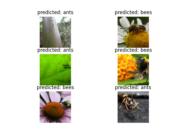
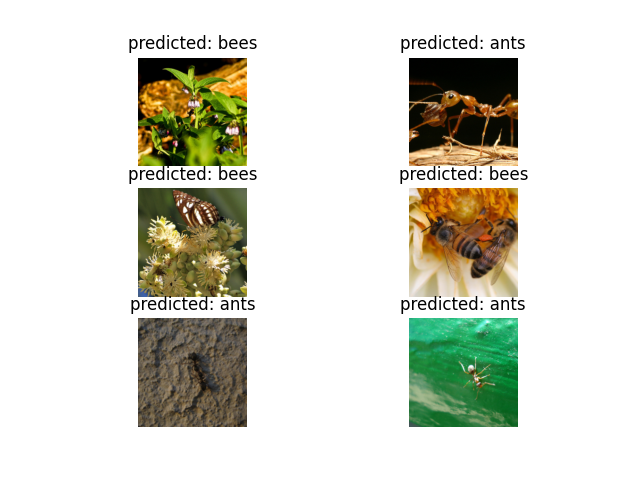
視覺化模型預測

顯示一些影像預測的通用函式

def visualize_model(model, num_images=6):
    was_training = model.training
    model.eval()
    images_so_far = 0
    fig = plt.figure()

    with torch.no_grad():
        for i, (inputs, labels) in enumerate(dataloaders['val']):
            inputs = inputs.to(device)
            labels = labels.to(device)

            outputs = model(inputs)
            _, preds = torch.max(outputs, 1)

            for j in range(inputs.size()[0]):
                images_so_far += 1
                ax = plt.subplot(num_images//2, 2, images_so_far)
                ax.axis('off')
                ax.set_title(f'predicted: {class_names[preds[j]]}')
                imshow(inputs.cpu().data[j])

                if images_so_far == num_images:
                    model.train(mode=was_training)
                    return
        model.train(mode=was_training)

微調 ConvNet

載入預訓練模型並重置最終全連線層。

model_ft = models.resnet18(weights='IMAGENET1K_V1')
num_ftrs = model_ft.fc.in_features
# Here the size of each output sample is set to 2.
# Alternatively, it can be generalized to ``nn.Linear(num_ftrs, len(class_names))``.
model_ft.fc = nn.Linear(num_ftrs, 2)

model_ft = model_ft.to(device)

criterion = nn.CrossEntropyLoss()

# Observe that all parameters are being optimized
optimizer_ft = optim.SGD(model_ft.parameters(), lr=0.001, momentum=0.9)

# Decay LR by a factor of 0.1 every 7 epochs
exp_lr_scheduler = lr_scheduler.StepLR(optimizer_ft, step_size=7, gamma=0.1)

Downloading: "https://download.pytorch.org/models/resnet18-f37072fd.pth" to /var/lib/ci-user/.cache/torch/hub/checkpoints/resnet18-f37072fd.pth

  0%|          | 0.00/44.7M [00:00<?, ?B/s]
 65%|######5   | 29.2M/44.7M [00:00<00:00, 301MB/s]
100%|##########| 44.7M/44.7M [00:00<00:00, 335MB/s]

訓練和評估

在 CPU 上大約需要 15-25 分鐘。在 GPU 上則不到一分鐘。

model_ft = train_model(model_ft, criterion, optimizer_ft, exp_lr_scheduler,
                       num_epochs=25)

Epoch 0/24
----------
train Loss: 0.4787 Acc: 0.7623
val Loss: 0.2826 Acc: 0.8824

Epoch 1/24
----------
train Loss: 0.5323 Acc: 0.7951
val Loss: 0.5748 Acc: 0.7712

Epoch 2/24
----------
train Loss: 0.4174 Acc: 0.8320
val Loss: 0.2629 Acc: 0.9150

Epoch 3/24
----------
train Loss: 0.5516 Acc: 0.7664
val Loss: 0.3715 Acc: 0.8693

Epoch 4/24
----------
train Loss: 0.3716 Acc: 0.8689
val Loss: 0.2691 Acc: 0.9020

Epoch 5/24
----------
train Loss: 0.4827 Acc: 0.7992
val Loss: 0.2696 Acc: 0.8824

Epoch 6/24
----------
train Loss: 0.3853 Acc: 0.8115
val Loss: 0.4517 Acc: 0.8366

Epoch 7/24
----------
train Loss: 0.3616 Acc: 0.8607
val Loss: 0.2149 Acc: 0.9216

Epoch 8/24
----------
train Loss: 0.2117 Acc: 0.9098
val Loss: 0.2153 Acc: 0.9216

Epoch 9/24
----------
train Loss: 0.2672 Acc: 0.8770
val Loss: 0.2565 Acc: 0.8954

Epoch 10/24
----------
train Loss: 0.3424 Acc: 0.8525
val Loss: 0.2022 Acc: 0.9281

Epoch 11/24
----------
train Loss: 0.3070 Acc: 0.8402
val Loss: 0.2594 Acc: 0.9085

Epoch 12/24
----------
train Loss: 0.2223 Acc: 0.8975
val Loss: 0.2480 Acc: 0.9020

Epoch 13/24
----------
train Loss: 0.3150 Acc: 0.8648
val Loss: 0.1974 Acc: 0.9216

Epoch 14/24
----------
train Loss: 0.2537 Acc: 0.9098
val Loss: 0.2640 Acc: 0.9150

Epoch 15/24
----------
train Loss: 0.2886 Acc: 0.8689
val Loss: 0.3004 Acc: 0.9150

Epoch 16/24
----------
train Loss: 0.2168 Acc: 0.8934
val Loss: 0.2329 Acc: 0.9085

Epoch 17/24
----------
train Loss: 0.2331 Acc: 0.9098
val Loss: 0.1952 Acc: 0.9216

Epoch 18/24
----------
train Loss: 0.2578 Acc: 0.9139
val Loss: 0.2462 Acc: 0.9150

Epoch 19/24
----------
train Loss: 0.2068 Acc: 0.9139
val Loss: 0.2290 Acc: 0.9085

Epoch 20/24
----------
train Loss: 0.2569 Acc: 0.8689
val Loss: 0.2089 Acc: 0.9085

Epoch 21/24
----------
train Loss: 0.2562 Acc: 0.8975
val Loss: 0.2546 Acc: 0.9150

Epoch 22/24
----------
train Loss: 0.3195 Acc: 0.8484
val Loss: 0.2214 Acc: 0.8954

Epoch 23/24
----------
train Loss: 0.2553 Acc: 0.8893
val Loss: 0.2295 Acc: 0.9150

Epoch 24/24
----------
train Loss: 0.2891 Acc: 0.8811
val Loss: 0.2033 Acc: 0.9216

Training complete in 0m 35s
Best val Acc: 0.928105

visualize_model(model_ft)

將 ConvNet 作為固定特徵提取器

在這裡，我們需要凍結除了最後一層之外的所有網路。我們需要設定 requires_grad = False 來凍結引數，以便在 backward() 中不計算梯度。

你可以在此處的文件中閱讀更多相關內容。

model_conv = torchvision.models.resnet18(weights='IMAGENET1K_V1')
for param in model_conv.parameters():
    param.requires_grad = False

# Parameters of newly constructed modules have requires_grad=True by default
num_ftrs = model_conv.fc.in_features
model_conv.fc = nn.Linear(num_ftrs, 2)

model_conv = model_conv.to(device)

criterion = nn.CrossEntropyLoss()

# Observe that only parameters of final layer are being optimized as
# opposed to before.
optimizer_conv = optim.SGD(model_conv.fc.parameters(), lr=0.001, momentum=0.9)

# Decay LR by a factor of 0.1 every 7 epochs
exp_lr_scheduler = lr_scheduler.StepLR(optimizer_conv, step_size=7, gamma=0.1)

訓練和評估

在 CPU 上，這大約是前一種情況所需時間的一半。這是預期的，因為大多數網路不需要計算梯度。然而，前向傳播仍然需要計算。

model_conv = train_model(model_conv, criterion, optimizer_conv,
                         exp_lr_scheduler, num_epochs=25)

Epoch 0/24
----------
train Loss: 0.6996 Acc: 0.6516
val Loss: 0.2014 Acc: 0.9346

Epoch 1/24
----------
train Loss: 0.4233 Acc: 0.8033
val Loss: 0.2655 Acc: 0.8758

Epoch 2/24
----------
train Loss: 0.4603 Acc: 0.7869
val Loss: 0.1847 Acc: 0.9477

Epoch 3/24
----------
train Loss: 0.3096 Acc: 0.8566
val Loss: 0.1747 Acc: 0.9477

Epoch 4/24
----------
train Loss: 0.4427 Acc: 0.8156
val Loss: 0.1630 Acc: 0.9477

Epoch 5/24
----------
train Loss: 0.5505 Acc: 0.7828
val Loss: 0.1642 Acc: 0.9477

Epoch 6/24
----------
train Loss: 0.3004 Acc: 0.8607
val Loss: 0.1744 Acc: 0.9542

Epoch 7/24
----------
train Loss: 0.4083 Acc: 0.8361
val Loss: 0.1892 Acc: 0.9412

Epoch 8/24
----------
train Loss: 0.4483 Acc: 0.7910
val Loss: 0.1984 Acc: 0.9477

Epoch 9/24
----------
train Loss: 0.3335 Acc: 0.8279
val Loss: 0.1942 Acc: 0.9412

Epoch 10/24
----------
train Loss: 0.2413 Acc: 0.8934
val Loss: 0.2000 Acc: 0.9477

Epoch 11/24
----------
train Loss: 0.3107 Acc: 0.8689
val Loss: 0.1801 Acc: 0.9412

Epoch 12/24
----------
train Loss: 0.3032 Acc: 0.8689
val Loss: 0.1669 Acc: 0.9477

Epoch 13/24
----------
train Loss: 0.3586 Acc: 0.8525
val Loss: 0.1900 Acc: 0.9477

Epoch 14/24
----------
train Loss: 0.2771 Acc: 0.8893
val Loss: 0.2318 Acc: 0.9216

Epoch 15/24
----------
train Loss: 0.3064 Acc: 0.8852
val Loss: 0.1909 Acc: 0.9477

Epoch 16/24
----------
train Loss: 0.4243 Acc: 0.8238
val Loss: 0.2227 Acc: 0.9346

Epoch 17/24
----------
train Loss: 0.3297 Acc: 0.8238
val Loss: 0.1916 Acc: 0.9412

Epoch 18/24
----------
train Loss: 0.4235 Acc: 0.8238
val Loss: 0.1766 Acc: 0.9477

Epoch 19/24
----------
train Loss: 0.2500 Acc: 0.8934
val Loss: 0.2003 Acc: 0.9477

Epoch 20/24
----------
train Loss: 0.2412 Acc: 0.8934
val Loss: 0.1821 Acc: 0.9477

Epoch 21/24
----------
train Loss: 0.3762 Acc: 0.8115
val Loss: 0.1842 Acc: 0.9412

Epoch 22/24
----------
train Loss: 0.3485 Acc: 0.8566
val Loss: 0.2166 Acc: 0.9281

Epoch 23/24
----------
train Loss: 0.3625 Acc: 0.8361
val Loss: 0.1747 Acc: 0.9412

Epoch 24/24
----------
train Loss: 0.3839 Acc: 0.8320
val Loss: 0.1768 Acc: 0.9412

Training complete in 0m 28s
Best val Acc: 0.954248

visualize_model(model_conv)

plt.ioff()
plt.show()

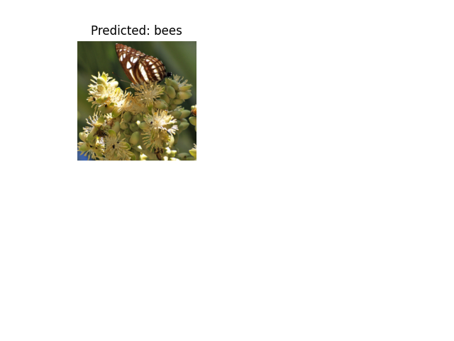
對自定義影像進行推理

使用訓練好的模型對自定義影像進行預測，並可視化預測的類別標籤以及影像。

def visualize_model_predictions(model,img_path):
    was_training = model.training
    model.eval()

    img = Image.open(img_path)
    img = data_transforms['val'](img)
    img = img.unsqueeze(0)
    img = img.to(device)

    with torch.no_grad():
        outputs = model(img)
        _, preds = torch.max(outputs, 1)

        ax = plt.subplot(2,2,1)
        ax.axis('off')
        ax.set_title(f'Predicted: {class_names[preds[0]]}')
        imshow(img.cpu().data[0])

        model.train(mode=was_training)

visualize_model_predictions(
    model_conv,
    img_path='data/hymenoptera_data/val/bees/72100438_73de9f17af.jpg'
)

plt.ioff()
plt.show()

進一步學習

如果你想了解更多關於遷移學習的應用，請檢視我們的計算機視覺量化遷移學習教程。