知識蒸餾教程

創建於： Aug 22, 2023 | 最後更新於： Jan 24, 2025 | 最後驗證於： Nov 05, 2024

作者: Alexandros Chariton

知識蒸餾是一種技術，它能夠在不損失有效性的前提下，將知識從大型、計算開銷大的模型轉移到小型模型。這使得模型能夠部署在算力較低的硬體上，評估更快且更高效。

在本教程中，我們將進行一系列實驗，旨在透過使用更強大的網路作為教師網路，來提高輕量級神經網路的準確性。輕量級網路的計算開銷和速度不會受到影響，我們的干預只集中在其權重上，而非其前向傳播過程。這項技術的應用可以在無人機或手機等裝置中找到。在本教程中，我們不使用任何外部包，因為所需的一切都可以在 torch 和 torchvision 中獲得。

在本教程中，您將學習

• 如何修改模型類以提取隱藏表示並將其用於進一步計算

• 如何修改 PyTorch 中的常規訓練迴圈，在例如用於分類任務的交叉熵損失之上，包含額外的損失函式

• 如何透過使用更復雜的模型作為教師網路來提高輕量級模型的效能

前提條件

• 1 個 GPU，4GB 視訊記憶體

• PyTorch v2.0 或更高版本

• CIFAR-10 資料集（由指令碼下載並儲存在名為 /data 的目錄中）

import torch
import torch.nn as nn
import torch.optim as optim
import torchvision.transforms as transforms
import torchvision.datasets as datasets

# Check if the current `accelerator <https://pytorch.com.tw/docs/stable/torch.html#accelerators>`__
# is available, and if not, use the CPU
device = torch.accelerator.current_accelerator().type if torch.accelerator.is_available() else "cpu"
print(f"Using {device} device")

Using cuda device

載入 CIFAR-10

CIFAR-10 是一個流行的影像資料集，包含十個類別。我們的目標是為每個輸入影像預測以下類別之一。

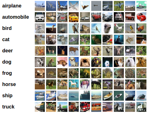
CIFAR-10 影像示例

輸入影像是 RGB 格式，因此它們有 3 個通道，大小為 32x32 畫素。基本上，每個影像由 3 x 32 x 32 = 3072 個介於 0 到 255 之間的數字描述。神經網路中的常見做法是歸一化輸入，這樣做有多種原因，包括避免常用啟用函式飽和以及提高數值穩定性。我們的歸一化過程包括減去每個通道的均值併除以標準差。張量“mean=[0.485, 0.456, 0.406]”和“std=[0.229, 0.224, 0.225]”已被計算出來，它們代表了 CIFAR-10 中預定義訓練集的每個通道的均值和標準差。注意，我們在測試集上也使用了這些值，而沒有從頭重新計算均值和標準差。這是因為網路是基於減去和除以上述數字後產生的特徵進行訓練的，我們希望保持一致性。此外，在實際應用中，我們將無法計算測試集的均值和標準差，因為根據我們的假設，那時這些資料將無法訪問。

最後一點，我們通常將這個保留集稱為驗證集，在最佳化模型在驗證集上的效能後，我們使用一個單獨的集合，稱為測試集。這樣做是為了避免基於對單一指標的貪婪和有偏最佳化來選擇模型。

# Below we are preprocessing data for CIFAR-10. We use an arbitrary batch size of 128.
transforms_cifar = transforms.Compose([
    transforms.ToTensor(),
    transforms.Normalize(mean=[0.485, 0.456, 0.406], std=[0.229, 0.224, 0.225]),
])

# Loading the CIFAR-10 dataset:
train_dataset = datasets.CIFAR10(root='./data', train=True, download=True, transform=transforms_cifar)
test_dataset = datasets.CIFAR10(root='./data', train=False, download=True, transform=transforms_cifar)

  0%|          | 0.00/170M [00:00<?, ?B/s]
  0%|          | 426k/170M [00:00<00:41, 4.10MB/s]
  3%|2         | 4.85M/170M [00:00<00:06, 27.2MB/s]
  6%|5         | 9.67M/170M [00:00<00:04, 36.6MB/s]
  8%|8         | 13.9M/170M [00:00<00:04, 38.6MB/s]
 10%|#         | 17.8M/170M [00:00<00:04, 33.1MB/s]
 12%|#2        | 21.2M/170M [00:00<00:04, 30.1MB/s]
 14%|#4        | 24.4M/170M [00:00<00:05, 28.6MB/s]
 16%|#6        | 27.3M/170M [00:00<00:05, 27.3MB/s]
 18%|#7        | 30.1M/170M [00:01<00:05, 26.7MB/s]
 19%|#9        | 32.8M/170M [00:01<00:05, 26.6MB/s]
 21%|##        | 35.5M/170M [00:01<00:05, 26.4MB/s]
 22%|##2       | 38.2M/170M [00:01<00:05, 26.1MB/s]
 24%|##4       | 41.0M/170M [00:01<00:04, 26.6MB/s]
 26%|##6       | 44.6M/170M [00:01<00:04, 29.2MB/s]
 28%|##8       | 47.9M/170M [00:01<00:04, 30.2MB/s]
 30%|###       | 51.4M/170M [00:01<00:03, 31.5MB/s]
 32%|###2      | 54.8M/170M [00:01<00:03, 31.9MB/s]
 34%|###4      | 58.2M/170M [00:01<00:03, 32.5MB/s]
 36%|###6      | 61.5M/170M [00:02<00:03, 32.6MB/s]
 38%|###8      | 64.8M/170M [00:02<00:03, 32.6MB/s]
 40%|###9      | 68.1M/170M [00:02<00:03, 32.3MB/s]
 42%|####1     | 71.3M/170M [00:02<00:03, 32.0MB/s]
 44%|####3     | 74.5M/170M [00:02<00:03, 31.7MB/s]
 46%|####5     | 77.7M/170M [00:02<00:03, 30.2MB/s]
 47%|####7     | 80.8M/170M [00:02<00:03, 27.3MB/s]
 49%|####9     | 83.6M/170M [00:02<00:03, 25.6MB/s]
 51%|#####     | 86.2M/170M [00:02<00:03, 24.4MB/s]
 52%|#####2    | 88.7M/170M [00:03<00:03, 23.8MB/s]
 53%|#####3    | 91.1M/170M [00:03<00:03, 23.3MB/s]
 55%|#####4    | 93.5M/170M [00:03<00:03, 22.9MB/s]
 56%|#####6    | 95.8M/170M [00:03<00:03, 22.7MB/s]
 58%|#####7    | 98.1M/170M [00:03<00:03, 22.4MB/s]
 59%|#####8    | 100M/170M [00:03<00:03, 22.3MB/s]
 60%|######    | 103M/170M [00:03<00:03, 22.2MB/s]
 61%|######1   | 105M/170M [00:03<00:02, 22.1MB/s]
 63%|######2   | 107M/170M [00:03<00:02, 21.9MB/s]
 64%|######4   | 109M/170M [00:04<00:02, 22.1MB/s]
 65%|######5   | 112M/170M [00:04<00:02, 21.9MB/s]
 67%|######6   | 114M/170M [00:04<00:02, 21.8MB/s]
 68%|######8   | 116M/170M [00:04<00:02, 21.9MB/s]
 69%|######9   | 118M/170M [00:04<00:02, 21.8MB/s]
 71%|#######   | 120M/170M [00:04<00:02, 21.9MB/s]
 72%|#######1  | 123M/170M [00:04<00:02, 21.8MB/s]
 73%|#######3  | 125M/170M [00:04<00:02, 21.8MB/s]
 75%|#######4  | 127M/170M [00:04<00:01, 21.8MB/s]
 76%|#######5  | 129M/170M [00:04<00:01, 21.8MB/s]
 77%|#######7  | 131M/170M [00:05<00:01, 21.5MB/s]
 78%|#######8  | 134M/170M [00:05<00:01, 21.4MB/s]
 80%|#######9  | 136M/170M [00:05<00:01, 21.5MB/s]
 81%|########  | 138M/170M [00:05<00:01, 21.2MB/s]
 82%|########2 | 140M/170M [00:05<00:01, 21.1MB/s]
 83%|########3 | 142M/170M [00:05<00:01, 20.9MB/s]
 85%|########4 | 144M/170M [00:05<00:01, 21.2MB/s]
 86%|########5 | 147M/170M [00:05<00:01, 21.1MB/s]
 87%|########7 | 149M/170M [00:05<00:01, 20.1MB/s]
 88%|########8 | 151M/170M [00:06<00:01, 19.0MB/s]
 90%|########9 | 153M/170M [00:06<00:00, 18.9MB/s]
 91%|######### | 155M/170M [00:06<00:00, 19.3MB/s]
 92%|#########1| 157M/170M [00:06<00:00, 18.8MB/s]
 93%|#########3| 159M/170M [00:06<00:00, 18.8MB/s]
 94%|#########4| 160M/170M [00:06<00:00, 17.7MB/s]
 95%|#########5| 162M/170M [00:06<00:00, 16.3MB/s]
 96%|#########6| 164M/170M [00:06<00:00, 15.3MB/s]
 97%|#########7| 166M/170M [00:06<00:00, 14.8MB/s]
 98%|#########7| 167M/170M [00:07<00:00, 14.4MB/s]
 99%|#########8| 169M/170M [00:07<00:00, 14.1MB/s]
100%|#########9| 170M/170M [00:07<00:00, 13.8MB/s]
100%|##########| 170M/170M [00:07<00:00, 23.3MB/s]

注意

本節僅適用於對快速獲得結果感興趣的 CPU 使用者。僅當您對小規模實驗感興趣時使用此選項。請記住，使用任何 GPU 程式碼都應該執行得相當快。僅從訓練/測試資料集中選擇前 num_images_to_keep 個影像

#from torch.utils.data import Subset
#num_images_to_keep = 2000
#train_dataset = Subset(train_dataset, range(min(num_images_to_keep, 50_000)))
#test_dataset = Subset(test_dataset, range(min(num_images_to_keep, 10_000)))

#Dataloaders
train_loader = torch.utils.data.DataLoader(train_dataset, batch_size=128, shuffle=True, num_workers=2)
test_loader = torch.utils.data.DataLoader(test_dataset, batch_size=128, shuffle=False, num_workers=2)

定義模型類和輔助函式

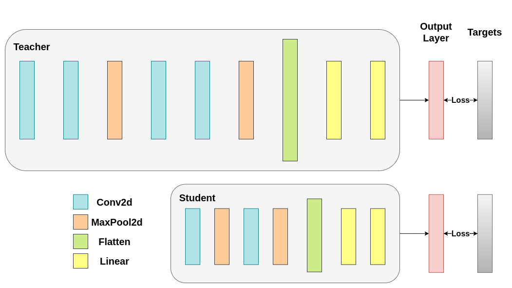
接下來，我們需要定義我們的模型類。這裡需要設定幾個使用者定義引數。我們使用兩種不同的架構，在實驗中保持濾波器數量固定，以確保公平比較。兩種架構都是卷積神經網路 (CNN)，具有不同數量的卷積層作為特徵提取器，後跟一個具有 10 個類別的分類器。學生網路的濾波器和神經元數量較少。

# Deeper neural network class to be used as teacher:
class DeepNN(nn.Module):
    def __init__(self, num_classes=10):
        super(DeepNN, self).__init__()
        self.features = nn.Sequential(
            nn.Conv2d(3, 128, kernel_size=3, padding=1),
            nn.ReLU(),
            nn.Conv2d(128, 64, kernel_size=3, padding=1),
            nn.ReLU(),
            nn.MaxPool2d(kernel_size=2, stride=2),
            nn.Conv2d(64, 64, kernel_size=3, padding=1),
            nn.ReLU(),
            nn.Conv2d(64, 32, kernel_size=3, padding=1),
            nn.ReLU(),
            nn.MaxPool2d(kernel_size=2, stride=2),
        )
        self.classifier = nn.Sequential(
            nn.Linear(2048, 512),
            nn.ReLU(),
            nn.Dropout(0.1),
            nn.Linear(512, num_classes)
        )

    def forward(self, x):
        x = self.features(x)
        x = torch.flatten(x, 1)
        x = self.classifier(x)
        return x

# Lightweight neural network class to be used as student:
class LightNN(nn.Module):
    def __init__(self, num_classes=10):
        super(LightNN, self).__init__()
        self.features = nn.Sequential(
            nn.Conv2d(3, 16, kernel_size=3, padding=1),
            nn.ReLU(),
            nn.MaxPool2d(kernel_size=2, stride=2),
            nn.Conv2d(16, 16, kernel_size=3, padding=1),
            nn.ReLU(),
            nn.MaxPool2d(kernel_size=2, stride=2),
        )
        self.classifier = nn.Sequential(
            nn.Linear(1024, 256),
            nn.ReLU(),
            nn.Dropout(0.1),
            nn.Linear(256, num_classes)
        )

    def forward(self, x):
        x = self.features(x)
        x = torch.flatten(x, 1)
        x = self.classifier(x)
        return x

我們使用 2 個函式來幫助我們在原始分類任務上產生和評估結果。其中一個函式稱為 train，接受以下引數

• model: 透過此函式訓練（更新權重）的模型例項。

• train_loader: 我們在上面定義了 train_loader，它的作用是將資料饋送到模型。

• epochs: 我們遍歷資料集的次數。

• learning_rate: 學習率決定了我們朝著收斂方向邁進的步長。步長過大或過小都可能有害。

• device: 確定執行工作負載的裝置。可以是 CPU 或 GPU，取決於可用性。

我們的測試函式類似，但會使用 test_loader 來載入測試集中的影像。

使用交叉熵訓練兩個網路。學生網路將用作基線：

def train(model, train_loader, epochs, learning_rate, device):
    criterion = nn.CrossEntropyLoss()
    optimizer = optim.Adam(model.parameters(), lr=learning_rate)

    model.train()

    for epoch in range(epochs):
        running_loss = 0.0
        for inputs, labels in train_loader:
            # inputs: A collection of batch_size images
            # labels: A vector of dimensionality batch_size with integers denoting class of each image
            inputs, labels = inputs.to(device), labels.to(device)

            optimizer.zero_grad()
            outputs = model(inputs)

            # outputs: Output of the network for the collection of images. A tensor of dimensionality batch_size x num_classes
            # labels: The actual labels of the images. Vector of dimensionality batch_size
            loss = criterion(outputs, labels)
            loss.backward()
            optimizer.step()

            running_loss += loss.item()

        print(f"Epoch {epoch+1}/{epochs}, Loss: {running_loss / len(train_loader)}")

def test(model, test_loader, device):
    model.to(device)
    model.eval()

    correct = 0
    total = 0

    with torch.no_grad():
        for inputs, labels in test_loader:
            inputs, labels = inputs.to(device), labels.to(device)

            outputs = model(inputs)
            _, predicted = torch.max(outputs.data, 1)

            total += labels.size(0)
            correct += (predicted == labels).sum().item()

    accuracy = 100 * correct / total
    print(f"Test Accuracy: {accuracy:.2f}%")
    return accuracy

交叉熵執行

為了可重複性，我們需要設定 torch 手動種子。我們使用不同的方法訓練網路，因此為了公平比較，最好用相同的權重初始化網路。首先使用交叉熵訓練教師網路

torch.manual_seed(42)
nn_deep = DeepNN(num_classes=10).to(device)
train(nn_deep, train_loader, epochs=10, learning_rate=0.001, device=device)
test_accuracy_deep = test(nn_deep, test_loader, device)

# Instantiate the lightweight network:
torch.manual_seed(42)
nn_light = LightNN(num_classes=10).to(device)

Epoch 1/10, Loss: 1.348291786125554
Epoch 2/10, Loss: 0.8802619594747149
Epoch 3/10, Loss: 0.6910638084344547
Epoch 4/10, Loss: 0.5453190243305148
Epoch 5/10, Loss: 0.4225382124600203
Epoch 6/10, Loss: 0.3179327983151921
Epoch 7/10, Loss: 0.22859162307532546
Epoch 8/10, Loss: 0.16856732934027377
Epoch 9/10, Loss: 0.14358678597318547
Epoch 10/10, Loss: 0.12967746109818407
Test Accuracy: 75.62%

我們再例項化一個輕量級網路模型來比較它們的效能。反向傳播對權重初始化很敏感，因此我們需要確保這兩個網路具有完全相同的初始化。

torch.manual_seed(42)
new_nn_light = LightNN(num_classes=10).to(device)

為了確保我們建立了第一個網路的副本，我們檢查其第一層的範數。如果匹配，我們可以放心地得出結論，這兩個網路確實是相同的。

# Print the norm of the first layer of the initial lightweight model
print("Norm of 1st layer of nn_light:", torch.norm(nn_light.features[0].weight).item())
# Print the norm of the first layer of the new lightweight model
print("Norm of 1st layer of new_nn_light:", torch.norm(new_nn_light.features[0].weight).item())

Norm of 1st layer of nn_light: 2.327361822128296
Norm of 1st layer of new_nn_light: 2.327361822128296

列印每個模型中的總引數數量

total_params_deep = "{:,}".format(sum(p.numel() for p in nn_deep.parameters()))
print(f"DeepNN parameters: {total_params_deep}")
total_params_light = "{:,}".format(sum(p.numel() for p in nn_light.parameters()))
print(f"LightNN parameters: {total_params_light}")

DeepNN parameters: 1,186,986
LightNN parameters: 267,738

使用交叉熵損失訓練並測試輕量級網路

train(nn_light, train_loader, epochs=10, learning_rate=0.001, device=device)
test_accuracy_light_ce = test(nn_light, test_loader, device)

Epoch 1/10, Loss: 1.4697812533439578
Epoch 2/10, Loss: 1.153727483871343
Epoch 3/10, Loss: 1.0198465607050435
Epoch 4/10, Loss: 0.9203303406000747
Epoch 5/10, Loss: 0.8472354605679622
Epoch 6/10, Loss: 0.7809330093891115
Epoch 7/10, Loss: 0.7178317027171249
Epoch 8/10, Loss: 0.660715803084776
Epoch 9/10, Loss: 0.6083721332537854
Epoch 10/10, Loss: 0.5571968615664851
Test Accuracy: 70.43%

正如我們所見，基於測試準確性，我們現在可以將用作教師網路的更深層網路與我們預期的學生網路進行比較。到目前為止，學生網路尚未與教師網路進行干預，因此這個效能是學生網路本身實現的。當前的指標可以透過以下行看到

print(f"Teacher accuracy: {test_accuracy_deep:.2f}%")
print(f"Student accuracy: {test_accuracy_light_ce:.2f}%")

Teacher accuracy: 75.62%
Student accuracy: 70.43%

知識蒸餾執行

現在，讓我們嘗試透過融入教師網路來提高學生網路的測試準確性。知識蒸餾是一種直接的技術，其基礎是兩個網路都輸出關於類別的機率分佈。因此，兩個網路共享相同數量的輸出神經元。該方法透過在傳統的交叉熵損失中加入一個額外的損失來實現，這個額外的損失基於教師網路的 softmax 輸出。其假設是，經過適當訓練的教師網路的輸出啟用攜帶了學生網路在訓練期間可以利用的額外資訊。原始研究表明，利用軟目標中較小機率的比率有助於實現深度神經網路的潛在目標，即在資料上建立一種相似性結構，將相似的物件對映得更近。例如，在 CIFAR-10 中，一輛卡車如果存在輪子，可能會被誤認為是汽車或飛機，但不太可能被誤認為是狗。因此，可以合理地假設有價值的資訊不僅存在於經過適當訓練的模型的最高預測中，還存在於整個輸出分佈中。然而，僅憑交叉熵無法充分利用這些資訊，因為非預測類別的啟用往往非常小，導致傳播的梯度無法有效地改變權重來構建這種理想的向量空間。

當我們繼續定義引入教師-學生動態的第一個輔助函式時，需要包含一些額外的引數

• T: 溫度，控制輸出分佈的平滑度。較大的 T 會導致更平滑的分佈，從而使較小的機率獲得更大的提升。

• soft_target_loss_weight: 分配給我們即將包含的額外目標的權重。

• ce_loss_weight: 分配給交叉熵的權重。調整這些權重會使網路傾向於最佳化其中任一目標。

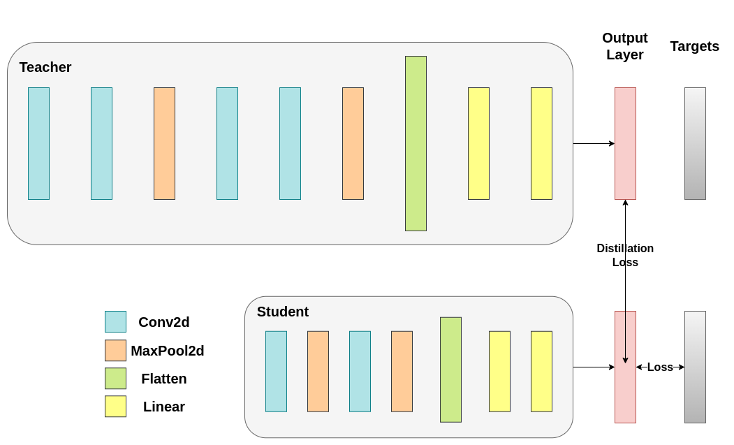
蒸餾損失是根據網路的 logits 計算的。它只向學生網路返回梯度：

def train_knowledge_distillation(teacher, student, train_loader, epochs, learning_rate, T, soft_target_loss_weight, ce_loss_weight, device):
    ce_loss = nn.CrossEntropyLoss()
    optimizer = optim.Adam(student.parameters(), lr=learning_rate)

    teacher.eval()  # Teacher set to evaluation mode
    student.train() # Student to train mode

    for epoch in range(epochs):
        running_loss = 0.0
        for inputs, labels in train_loader:
            inputs, labels = inputs.to(device), labels.to(device)

            optimizer.zero_grad()

            # Forward pass with the teacher model - do not save gradients here as we do not change the teacher's weights
            with torch.no_grad():
                teacher_logits = teacher(inputs)

            # Forward pass with the student model
            student_logits = student(inputs)

            #Soften the student logits by applying softmax first and log() second
            soft_targets = nn.functional.softmax(teacher_logits / T, dim=-1)
            soft_prob = nn.functional.log_softmax(student_logits / T, dim=-1)

            # Calculate the soft targets loss. Scaled by T**2 as suggested by the authors of the paper "Distilling the knowledge in a neural network"
            soft_targets_loss = torch.sum(soft_targets * (soft_targets.log() - soft_prob)) / soft_prob.size()[0] * (T**2)

            # Calculate the true label loss
            label_loss = ce_loss(student_logits, labels)

            # Weighted sum of the two losses
            loss = soft_target_loss_weight * soft_targets_loss + ce_loss_weight * label_loss

            loss.backward()
            optimizer.step()

            running_loss += loss.item()

        print(f"Epoch {epoch+1}/{epochs}, Loss: {running_loss / len(train_loader)}")

# Apply ``train_knowledge_distillation`` with a temperature of 2. Arbitrarily set the weights to 0.75 for CE and 0.25 for distillation loss.
train_knowledge_distillation(teacher=nn_deep, student=new_nn_light, train_loader=train_loader, epochs=10, learning_rate=0.001, T=2, soft_target_loss_weight=0.25, ce_loss_weight=0.75, device=device)
test_accuracy_light_ce_and_kd = test(new_nn_light, test_loader, device)

# Compare the student test accuracy with and without the teacher, after distillation
print(f"Teacher accuracy: {test_accuracy_deep:.2f}%")
print(f"Student accuracy without teacher: {test_accuracy_light_ce:.2f}%")
print(f"Student accuracy with CE + KD: {test_accuracy_light_ce_and_kd:.2f}%")

Epoch 1/10, Loss: 2.386750131921695
Epoch 2/10, Loss: 1.868185037237299
Epoch 3/10, Loss: 1.642685822513707
Epoch 4/10, Loss: 1.484524897602208
Epoch 5/10, Loss: 1.3599990208435546
Epoch 6/10, Loss: 1.2424575910543847
Epoch 7/10, Loss: 1.147350205942188
Epoch 8/10, Loss: 1.0649026226814446
Epoch 9/10, Loss: 0.9886922711301642
Epoch 10/10, Loss: 0.9178902323898452
Test Accuracy: 70.48%
Teacher accuracy: 75.62%
Student accuracy without teacher: 70.43%
Student accuracy with CE + KD: 70.48%

餘弦損失最小化執行

您可以隨意調整控制 softmax 函式軟化程度的溫度引數和損失係數。在神經網路中，很容易為主目標新增額外的損失函式，以實現更好的泛化等目標。讓我們嘗試為學生網路包含一個目標，但現在我們將重點放在它們的隱藏狀態，而不是輸出層。我們的目標是透過包含一個樸素的損失函式，將資訊從教師網路的表示傳遞給學生網路。這個損失函式的最小化意味著隨後傳遞給分類器的扁平化向量隨著損失的減小變得更相似。當然，教師網路不會更新其權重，因此最小化僅取決於學生網路的權重。這種方法背後的原理是，我們假設教師模型具有更好的內部表示，學生網路在沒有外部干預的情況下不太可能達到這種表示，因此我們人工地推動學生網路模仿教師網路的內部表示。然而，這是否最終會幫助學生網路並不簡單，因為將輕量級網路推向這個點可能是一件好事，前提是我們找到了一個能帶來更好測試準確性的內部表示，但也可能有害，因為網路具有不同的架構，學生網路沒有與教師網路相同的學習能力。換句話說，學生和教師的這兩個向量沒有理由在每個元件上完全匹配。學生網路可以達到一個內部表示，它是教師網路表示的一個排列，並且效率相同。儘管如此，我們仍然可以進行一個快速實驗來弄清楚這種方法的影響。我們將使用 CosineEmbeddingLoss，它的公式如下

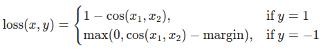
CosineEmbeddingLoss 公式

顯然，我們首先需要解決一個問題。當我們對輸出層應用蒸餾時，我們提到兩個網路都具有相同數量的神經元，等於類別的數量。然而，對於卷積層之後的層來說並非如此。在這裡，在最終卷積層展平後，教師網路比學生網路擁有更多神經元。我們的損失函式接受兩個維度相同的向量作為輸入，因此我們需要以某種方式匹配它們。我們將透過在教師網路的卷積層之後包含一個平均池化層來解決這個問題，以減小其維度，使其與學生網路的維度匹配。

為了繼續，我們將修改我們的模型類，或建立新的模型類。現在，前向傳播函式不僅返回網路的 logits，還返回卷積層之後的展平隱藏表示。我們為修改後的教師網路包含了上述池化層。

class ModifiedDeepNNCosine(nn.Module):
    def __init__(self, num_classes=10):
        super(ModifiedDeepNNCosine, self).__init__()
        self.features = nn.Sequential(
            nn.Conv2d(3, 128, kernel_size=3, padding=1),
            nn.ReLU(),
            nn.Conv2d(128, 64, kernel_size=3, padding=1),
            nn.ReLU(),
            nn.MaxPool2d(kernel_size=2, stride=2),
            nn.Conv2d(64, 64, kernel_size=3, padding=1),
            nn.ReLU(),
            nn.Conv2d(64, 32, kernel_size=3, padding=1),
            nn.ReLU(),
            nn.MaxPool2d(kernel_size=2, stride=2),
        )
        self.classifier = nn.Sequential(
            nn.Linear(2048, 512),
            nn.ReLU(),
            nn.Dropout(0.1),
            nn.Linear(512, num_classes)
        )

    def forward(self, x):
        x = self.features(x)
        flattened_conv_output = torch.flatten(x, 1)
        x = self.classifier(flattened_conv_output)
        flattened_conv_output_after_pooling = torch.nn.functional.avg_pool1d(flattened_conv_output, 2)
        return x, flattened_conv_output_after_pooling

# Create a similar student class where we return a tuple. We do not apply pooling after flattening.
class ModifiedLightNNCosine(nn.Module):
    def __init__(self, num_classes=10):
        super(ModifiedLightNNCosine, self).__init__()
        self.features = nn.Sequential(
            nn.Conv2d(3, 16, kernel_size=3, padding=1),
            nn.ReLU(),
            nn.MaxPool2d(kernel_size=2, stride=2),
            nn.Conv2d(16, 16, kernel_size=3, padding=1),
            nn.ReLU(),
            nn.MaxPool2d(kernel_size=2, stride=2),
        )
        self.classifier = nn.Sequential(
            nn.Linear(1024, 256),
            nn.ReLU(),
            nn.Dropout(0.1),
            nn.Linear(256, num_classes)
        )

    def forward(self, x):
        x = self.features(x)
        flattened_conv_output = torch.flatten(x, 1)
        x = self.classifier(flattened_conv_output)
        return x, flattened_conv_output

# We do not have to train the modified deep network from scratch of course, we just load its weights from the trained instance
modified_nn_deep = ModifiedDeepNNCosine(num_classes=10).to(device)
modified_nn_deep.load_state_dict(nn_deep.state_dict())

# Once again ensure the norm of the first layer is the same for both networks
print("Norm of 1st layer for deep_nn:", torch.norm(nn_deep.features[0].weight).item())
print("Norm of 1st layer for modified_deep_nn:", torch.norm(modified_nn_deep.features[0].weight).item())

# Initialize a modified lightweight network with the same seed as our other lightweight instances. This will be trained from scratch to examine the effectiveness of cosine loss minimization.
torch.manual_seed(42)
modified_nn_light = ModifiedLightNNCosine(num_classes=10).to(device)
print("Norm of 1st layer:", torch.norm(modified_nn_light.features[0].weight).item())

Norm of 1st layer for deep_nn: 7.503714084625244
Norm of 1st layer for modified_deep_nn: 7.503714084625244
Norm of 1st layer: 2.327361822128296

自然地，我們需要更改訓練迴圈，因為現在模型返回一個元組 (logits, hidden_representation)。使用一個示例輸入張量，我們可以列印它們的形狀。

# Create a sample input tensor
sample_input = torch.randn(128, 3, 32, 32).to(device) # Batch size: 128, Filters: 3, Image size: 32x32

# Pass the input through the student
logits, hidden_representation = modified_nn_light(sample_input)

# Print the shapes of the tensors
print("Student logits shape:", logits.shape) # batch_size x total_classes
print("Student hidden representation shape:", hidden_representation.shape) # batch_size x hidden_representation_size

# Pass the input through the teacher
logits, hidden_representation = modified_nn_deep(sample_input)

# Print the shapes of the tensors
print("Teacher logits shape:", logits.shape) # batch_size x total_classes
print("Teacher hidden representation shape:", hidden_representation.shape) # batch_size x hidden_representation_size

Student logits shape: torch.Size([128, 10])
Student hidden representation shape: torch.Size([128, 1024])
Teacher logits shape: torch.Size([128, 10])
Teacher hidden representation shape: torch.Size([128, 1024])

在我們的例子中，hidden_representation_size 是 1024。這是學生網路最終卷積層的展平特徵圖，如您所見，它是其分類器的輸入。對於教師網路也是 1024，因為我們使用 avg_pool1d 將其從 2048 變為了 1024。這裡應用的損失僅影響學生網路在損失計算之前的權重。換句話說，它不影響學生網路的分類器。修改後的訓練迴圈如下

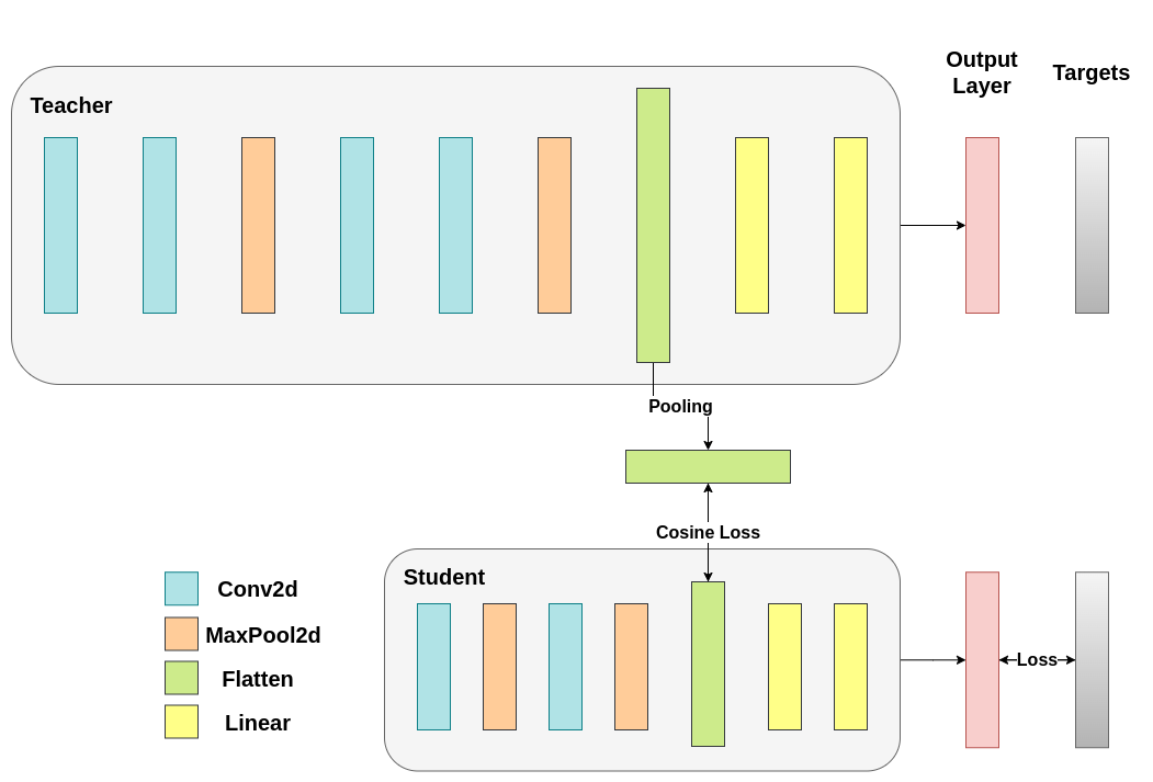
在餘弦損失最小化中，我們希望透過向學生網路返回梯度來最大化兩個表示的餘弦相似度：

def train_cosine_loss(teacher, student, train_loader, epochs, learning_rate, hidden_rep_loss_weight, ce_loss_weight, device):
    ce_loss = nn.CrossEntropyLoss()
    cosine_loss = nn.CosineEmbeddingLoss()
    optimizer = optim.Adam(student.parameters(), lr=learning_rate)

    teacher.to(device)
    student.to(device)
    teacher.eval()  # Teacher set to evaluation mode
    student.train() # Student to train mode

    for epoch in range(epochs):
        running_loss = 0.0
        for inputs, labels in train_loader:
            inputs, labels = inputs.to(device), labels.to(device)

            optimizer.zero_grad()

            # Forward pass with the teacher model and keep only the hidden representation
            with torch.no_grad():
                _, teacher_hidden_representation = teacher(inputs)

            # Forward pass with the student model
            student_logits, student_hidden_representation = student(inputs)

            # Calculate the cosine loss. Target is a vector of ones. From the loss formula above we can see that is the case where loss minimization leads to cosine similarity increase.
            hidden_rep_loss = cosine_loss(student_hidden_representation, teacher_hidden_representation, target=torch.ones(inputs.size(0)).to(device))

            # Calculate the true label loss
            label_loss = ce_loss(student_logits, labels)

            # Weighted sum of the two losses
            loss = hidden_rep_loss_weight * hidden_rep_loss + ce_loss_weight * label_loss

            loss.backward()
            optimizer.step()

            running_loss += loss.item()

        print(f"Epoch {epoch+1}/{epochs}, Loss: {running_loss / len(train_loader)}")

由於同樣的原因，我們需要修改我們的測試函式。在這裡，我們忽略了模型返回的隱藏表示。

def test_multiple_outputs(model, test_loader, device):
    model.to(device)
    model.eval()

    correct = 0
    total = 0

    with torch.no_grad():
        for inputs, labels in test_loader:
            inputs, labels = inputs.to(device), labels.to(device)

            outputs, _ = model(inputs) # Disregard the second tensor of the tuple
            _, predicted = torch.max(outputs.data, 1)

            total += labels.size(0)
            correct += (predicted == labels).sum().item()

    accuracy = 100 * correct / total
    print(f"Test Accuracy: {accuracy:.2f}%")
    return accuracy

在這種情況下，我們可以很容易地將知識蒸餾和餘弦損失最小化包含在同一個函式中。在教師-學生正規化中，結合多種方法來獲得更好的效能是常見的。現在，我們可以執行一個簡單的訓練-測試會話。

# Train and test the lightweight network with cross entropy loss
train_cosine_loss(teacher=modified_nn_deep, student=modified_nn_light, train_loader=train_loader, epochs=10, learning_rate=0.001, hidden_rep_loss_weight=0.25, ce_loss_weight=0.75, device=device)
test_accuracy_light_ce_and_cosine_loss = test_multiple_outputs(modified_nn_light, test_loader, device)

Epoch 1/10, Loss: 1.3048658852686967
Epoch 2/10, Loss: 1.0663291737246696
Epoch 3/10, Loss: 0.9672873822014655
Epoch 4/10, Loss: 0.8923313494228646
Epoch 5/10, Loss: 0.8383791920779001
Epoch 6/10, Loss: 0.7914473272650443
Epoch 7/10, Loss: 0.7511683412829934
Epoch 8/10, Loss: 0.7156466943833529
Epoch 9/10, Loss: 0.6772932203681877
Epoch 10/10, Loss: 0.6502810129729073
Test Accuracy: 70.76%

中間迴歸器執行

我們樸素的最小化方法並不能保證更好的結果，原因有幾個，其中之一是向量的維度。對於高維向量，餘弦相似度通常比歐幾里得距離效果更好，但我們處理的是每個向量有 1024 個分量，因此更難提取有意義的相似性。此外，正如我們所提到的，理論上並不支援推動教師網路和學生網路的隱藏表示完全匹配。沒有充分的理由說明我們應該追求這些向量的 1:1 匹配。我們將提供最後一個訓練干預的例子，即包含一個額外的網路，稱為迴歸器（regressor）。目標是首先提取教師網路在卷積層後的特徵圖，然後提取學生網路在卷積層後的特徵圖，最後嘗試匹配這些特徵圖。然而，這一次，我們將在網路之間引入一個迴歸器來促進匹配過程。迴歸器將是可訓練的，並且理想情況下會比我們樸素的餘弦損失最小化方案做得更好。它的主要工作是匹配這些特徵圖的維度，以便我們能夠在教師網路和學生網路之間正確定義一個損失函式。定義這樣的損失函式提供了一條教學“路徑”，它基本上是一個反向傳播梯度以改變學生權重的流程。重點關注我們原始網路中每個分類器之前的卷積層的輸出，我們得到以下形狀

# Pass the sample input only from the convolutional feature extractor
convolutional_fe_output_student = nn_light.features(sample_input)
convolutional_fe_output_teacher = nn_deep.features(sample_input)

# Print their shapes
print("Student's feature extractor output shape: ", convolutional_fe_output_student.shape)
print("Teacher's feature extractor output shape: ", convolutional_fe_output_teacher.shape)

Student's feature extractor output shape:  torch.Size([128, 16, 8, 8])
Teacher's feature extractor output shape:  torch.Size([128, 32, 8, 8])

教師網路有 32 個濾波器，學生網路有 16 個濾波器。我們將包含一個可訓練層，將學生網路的特徵圖轉換為教師網路的特徵圖形狀。實踐中，我們修改輕量級類，使其在中間迴歸器後返回隱藏狀態，該回歸器匹配卷積特徵圖的大小；而教師類則返回最終卷積層（不帶池化或展平）的輸出。

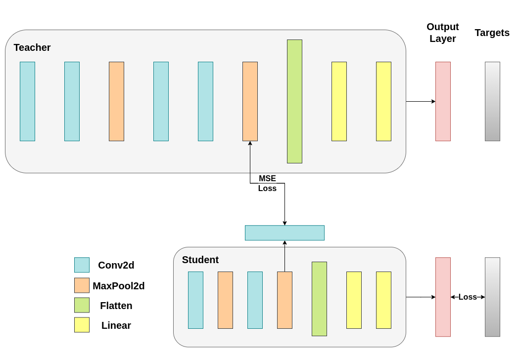
可訓練層匹配中間張量的形狀，並且均方誤差 (MSE) 被正確定義：

class ModifiedDeepNNRegressor(nn.Module):
    def __init__(self, num_classes=10):
        super(ModifiedDeepNNRegressor, self).__init__()
        self.features = nn.Sequential(
            nn.Conv2d(3, 128, kernel_size=3, padding=1),
            nn.ReLU(),
            nn.Conv2d(128, 64, kernel_size=3, padding=1),
            nn.ReLU(),
            nn.MaxPool2d(kernel_size=2, stride=2),
            nn.Conv2d(64, 64, kernel_size=3, padding=1),
            nn.ReLU(),
            nn.Conv2d(64, 32, kernel_size=3, padding=1),
            nn.ReLU(),
            nn.MaxPool2d(kernel_size=2, stride=2),
        )
        self.classifier = nn.Sequential(
            nn.Linear(2048, 512),
            nn.ReLU(),
            nn.Dropout(0.1),
            nn.Linear(512, num_classes)
        )

    def forward(self, x):
        x = self.features(x)
        conv_feature_map = x
        x = torch.flatten(x, 1)
        x = self.classifier(x)
        return x, conv_feature_map

class ModifiedLightNNRegressor(nn.Module):
    def __init__(self, num_classes=10):
        super(ModifiedLightNNRegressor, self).__init__()
        self.features = nn.Sequential(
            nn.Conv2d(3, 16, kernel_size=3, padding=1),
            nn.ReLU(),
            nn.MaxPool2d(kernel_size=2, stride=2),
            nn.Conv2d(16, 16, kernel_size=3, padding=1),
            nn.ReLU(),
            nn.MaxPool2d(kernel_size=2, stride=2),
        )
        # Include an extra regressor (in our case linear)
        self.regressor = nn.Sequential(
            nn.Conv2d(16, 32, kernel_size=3, padding=1)
        )
        self.classifier = nn.Sequential(
            nn.Linear(1024, 256),
            nn.ReLU(),
            nn.Dropout(0.1),
            nn.Linear(256, num_classes)
        )

    def forward(self, x):
        x = self.features(x)
        regressor_output = self.regressor(x)
        x = torch.flatten(x, 1)
        x = self.classifier(x)
        return x, regressor_output

之後，我們必須再次更新我們的訓練迴圈。這一次，我們提取學生網路的迴歸器輸出和教師網路的特徵圖，計算這些張量的 MSE（它們的形狀完全相同，因此定義正確），並在該損失的基礎上反向傳播梯度，此外還有分類任務的常規交叉熵損失。

def train_mse_loss(teacher, student, train_loader, epochs, learning_rate, feature_map_weight, ce_loss_weight, device):
    ce_loss = nn.CrossEntropyLoss()
    mse_loss = nn.MSELoss()
    optimizer = optim.Adam(student.parameters(), lr=learning_rate)

    teacher.to(device)
    student.to(device)
    teacher.eval()  # Teacher set to evaluation mode
    student.train() # Student to train mode

    for epoch in range(epochs):
        running_loss = 0.0
        for inputs, labels in train_loader:
            inputs, labels = inputs.to(device), labels.to(device)

            optimizer.zero_grad()

            # Again ignore teacher logits
            with torch.no_grad():
                _, teacher_feature_map = teacher(inputs)

            # Forward pass with the student model
            student_logits, regressor_feature_map = student(inputs)

            # Calculate the loss
            hidden_rep_loss = mse_loss(regressor_feature_map, teacher_feature_map)

            # Calculate the true label loss
            label_loss = ce_loss(student_logits, labels)

            # Weighted sum of the two losses
            loss = feature_map_weight * hidden_rep_loss + ce_loss_weight * label_loss

            loss.backward()
            optimizer.step()

            running_loss += loss.item()

        print(f"Epoch {epoch+1}/{epochs}, Loss: {running_loss / len(train_loader)}")

# Notice how our test function remains the same here with the one we used in our previous case. We only care about the actual outputs because we measure accuracy.

# Initialize a ModifiedLightNNRegressor
torch.manual_seed(42)
modified_nn_light_reg = ModifiedLightNNRegressor(num_classes=10).to(device)

# We do not have to train the modified deep network from scratch of course, we just load its weights from the trained instance
modified_nn_deep_reg = ModifiedDeepNNRegressor(num_classes=10).to(device)
modified_nn_deep_reg.load_state_dict(nn_deep.state_dict())

# Train and test once again
train_mse_loss(teacher=modified_nn_deep_reg, student=modified_nn_light_reg, train_loader=train_loader, epochs=10, learning_rate=0.001, feature_map_weight=0.25, ce_loss_weight=0.75, device=device)
test_accuracy_light_ce_and_mse_loss = test_multiple_outputs(modified_nn_light_reg, test_loader, device)

Epoch 1/10, Loss: 1.6814098352056634
Epoch 2/10, Loss: 1.3158039458267523
Epoch 3/10, Loss: 1.1743099965402841
Epoch 4/10, Loss: 1.0804673418059678
Epoch 5/10, Loss: 1.0056396507850998
Epoch 6/10, Loss: 0.9448006615004576
Epoch 7/10, Loss: 0.8926408891482731
Epoch 8/10, Loss: 0.842213883119471
Epoch 9/10, Loss: 0.8003371124682219
Epoch 10/10, Loss: 0.7620166893810263
Test Accuracy: 71.02%

預計最後一種方法會比 CosineLoss 效果更好，因為現在我們在教師網路和學生網路之間允許了一個可訓練層，這給了學生網路一些學習的餘地，而不是強制學生網路複製教師網路的表示。包含額外的網路是基於提示的蒸餾（hint-based distillation）背後的思想。

print(f"Teacher accuracy: {test_accuracy_deep:.2f}%")
print(f"Student accuracy without teacher: {test_accuracy_light_ce:.2f}%")
print(f"Student accuracy with CE + KD: {test_accuracy_light_ce_and_kd:.2f}%")
print(f"Student accuracy with CE + CosineLoss: {test_accuracy_light_ce_and_cosine_loss:.2f}%")
print(f"Student accuracy with CE + RegressorMSE: {test_accuracy_light_ce_and_mse_loss:.2f}%")

Teacher accuracy: 75.62%
Student accuracy without teacher: 70.43%
Student accuracy with CE + KD: 70.48%
Student accuracy with CE + CosineLoss: 70.76%
Student accuracy with CE + RegressorMSE: 71.02%

結論

上述方法均不會增加網路的引數數量或推理時間，因此效能提升的代價僅是在訓練期間計算梯度所帶來的微小開銷。在機器學習應用中，我們主要關注推理時間，因為訓練發生在模型部署之前。如果我們的輕量級模型對於部署仍然過重，我們可以應用不同的思路，例如訓練後量化。附加損失可以應用於許多工，而不僅僅是分類，並且你可以試驗諸如係數（coefficients）、溫度（temperature）或神經元數量（number of neurons）等量。歡迎調整上述教程中的任何數值，但請記住，如果你更改神經元/濾波器（filters）的數量，則很可能會發生形狀不匹配（shape mismatch）。

更多資訊請參閱：

• Hinton, G., Vinyals, O., Dean, J.: Distilling the knowledge in a neural network. In: Neural Information Processing System Deep Learning Workshop (2015)

• Romero, A., Ballas, N., Kahou, S.E., Chassang, A., Gatta, C., Bengio, Y.: Fitnets: Hints for thin deep nets. In: Proceedings of the International Conference on Learning Representations (2015)