使用自定義函式進行雙重反向傳播

創建於：2021 年 8 月 13 日 | 最後更新：2021 年 8 月 13 日 | 最後驗證：2024 年 11 月 05 日

有時，在反向圖上執行兩次反向傳播很有用，例如計算高階梯度。然而，支援雙重反向傳播需要對 autograd 有所瞭解並加以注意。僅支援一次反向傳播的函式不一定能夠支援雙重反向傳播。在本教程中，我們將展示如何編寫一個支援雙重反向傳播的自定義 autograd 函式，並指出一些需要注意的事項。

在編寫支援雙重反向傳播的自定義 autograd 函式時，瞭解在自定義函式中執行的操作何時會被 autograd 記錄、何時不會被記錄，以及最重要的是 save_for_backward 如何與這一切協同工作，這一點非常重要。

自定義函式以兩種方式隱式影響梯度模式：

• 在前向傳播期間，autograd 不會記錄在前向函式中執行的任何操作的圖。當前向傳播完成後，自定義函式的反向函式將成為前向傳播的每個輸出的 grad_fn。

• 在反向傳播期間，如果指定了 `create_graph`，autograd 會記錄用於計算反向傳播的計算圖。

接下來，為了理解 save_for_backward 如何與上述內容互動，我們可以探討幾個示例。

儲存輸入

考慮這個簡單的平方函式。它儲存輸入張量用於反向傳播。當 autograd 能夠在反向傳播過程中記錄操作時，雙重反向傳播會自動工作，因此當我們儲存輸入用於反向傳播時，通常無需擔心，因為如果輸入是任何需要梯度的張量的函式，它應該具有 grad_fn。這使得梯度能夠正確傳播。

import torch

class Square(torch.autograd.Function):
    @staticmethod
    def forward(ctx, x):
        # Because we are saving one of the inputs use `save_for_backward`
        # Save non-tensors and non-inputs/non-outputs directly on ctx
        ctx.save_for_backward(x)
        return x**2

    @staticmethod
    def backward(ctx, grad_out):
        # A function support double backward automatically if autograd
        # is able to record the computations performed in backward
        x, = ctx.saved_tensors
        return grad_out * 2 * x

# Use double precision because finite differencing method magnifies errors
x = torch.rand(3, 3, requires_grad=True, dtype=torch.double)
torch.autograd.gradcheck(Square.apply, x)
# Use gradcheck to verify second-order derivatives
torch.autograd.gradgradcheck(Square.apply, x)

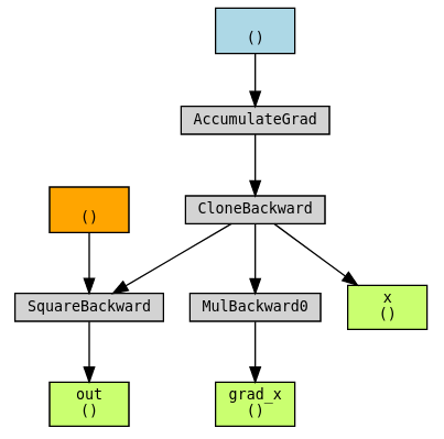
我們可以使用 torchviz 視覺化圖，以瞭解其工作原理。

import torchviz

x = torch.tensor(1., requires_grad=True).clone()
out = Square.apply(x)
grad_x, = torch.autograd.grad(out, x, create_graph=True)
torchviz.make_dot((grad_x, x, out), {"grad_x": grad_x, "x": x, "out": out})

我們可以看到，關於 x 的梯度本身是 x 的函式 (dout/dx = 2x)，並且這個函式的圖已經正確構建。

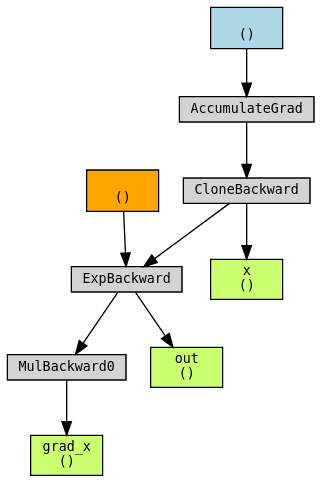
儲存輸出

上一個示例的一個微小變體是儲存輸出而不是輸入。其機制類似，因為輸出也與 grad_fn 相關聯。

class Exp(torch.autograd.Function):
    # Simple case where everything goes well
    @staticmethod
    def forward(ctx, x):
        # This time we save the output
        result = torch.exp(x)
        # Note that we should use `save_for_backward` here when
        # the tensor saved is an ouptut (or an input).
        ctx.save_for_backward(result)
        return result

    @staticmethod
    def backward(ctx, grad_out):
        result, = ctx.saved_tensors
        return result * grad_out

x = torch.tensor(1., requires_grad=True, dtype=torch.double).clone()
# Validate our gradients using gradcheck
torch.autograd.gradcheck(Exp.apply, x)
torch.autograd.gradgradcheck(Exp.apply, x)

使用 torchviz 視覺化圖。

out = Exp.apply(x)
grad_x, = torch.autograd.grad(out, x, create_graph=True)
torchviz.make_dot((grad_x, x, out), {"grad_x": grad_x, "x": x, "out": out})

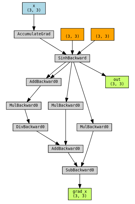
儲存中間結果

更棘手的情況是需要儲存中間結果。我們透過實現以下函式來演示這種情況：

\[sinh(x) := \frac{e^x - e^{-x}}{2} \]

由於 sinh 的導數是 cosh，因此在反向計算中重用前向傳播中的兩個中間結果 exp(x) 和 exp(-x) 可能會很有用。

然而，中間結果不應直接儲存並在反向傳播中使用。由於前向傳播在 no-grad 模式下執行，如果前向傳播的中間結果用於在反向傳播中計算梯度，那麼梯度的反向圖將不會包含計算中間結果的操作。這將導致不正確的梯度。

class Sinh(torch.autograd.Function):
    @staticmethod
    def forward(ctx, x):
        expx = torch.exp(x)
        expnegx = torch.exp(-x)
        ctx.save_for_backward(expx, expnegx)
        # In order to be able to save the intermediate results, a trick is to
        # include them as our outputs, so that the backward graph is constructed
        return (expx - expnegx) / 2, expx, expnegx

    @staticmethod
    def backward(ctx, grad_out, _grad_out_exp, _grad_out_negexp):
        expx, expnegx = ctx.saved_tensors
        grad_input = grad_out * (expx + expnegx) / 2
        # We cannot skip accumulating these even though we won't use the outputs
        # directly. They will be used later in the second backward.
        grad_input += _grad_out_exp * expx
        grad_input -= _grad_out_negexp * expnegx
        return grad_input

def sinh(x):
    # Create a wrapper that only returns the first output
    return Sinh.apply(x)[0]

x = torch.rand(3, 3, requires_grad=True, dtype=torch.double)
torch.autograd.gradcheck(sinh, x)
torch.autograd.gradgradcheck(sinh, x)

使用 torchviz 視覺化圖。

out = sinh(x)
grad_x, = torch.autograd.grad(out.sum(), x, create_graph=True)
torchviz.make_dot((grad_x, x, out), params={"grad_x": grad_x, "x": x, "out": out})

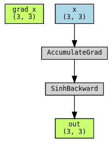
儲存中間結果：不應做的事情

現在我們展示如果不將中間結果作為輸出返回時會發生什麼：grad_x 甚至不會有反向圖，因為它完全是 exp 和 expnegx 的函式，而它們不需要梯度。

class SinhBad(torch.autograd.Function):
    # This is an example of what NOT to do!
    @staticmethod
    def forward(ctx, x):
        expx = torch.exp(x)
        expnegx = torch.exp(-x)
        ctx.expx = expx
        ctx.expnegx = expnegx
        return (expx - expnegx) / 2

    @staticmethod
    def backward(ctx, grad_out):
        expx = ctx.expx
        expnegx = ctx.expnegx
        grad_input = grad_out * (expx + expnegx) / 2
        return grad_input

使用 torchviz 視覺化圖。注意 grad_x 不在圖中！

out = SinhBad.apply(x)
grad_x, = torch.autograd.grad(out.sum(), x, create_graph=True)
torchviz.make_dot((grad_x, x, out), params={"grad_x": grad_x, "x": x, "out": out})

當反向傳播未被跟蹤時

最後，讓我們考慮一個 autograd 可能完全無法跟蹤函式反向傳播梯度的示例。我們可以設想 cube_backward 是一個可能需要 SciPy 或 NumPy 等非 PyTorch 庫的函式，或者寫成一個 C++ 擴充套件。這裡演示的解決方案是建立另一個自定義函式 CubeBackward，並在其中手動指定 cube_backward 的反向傳播！

def cube_forward(x):
    return x**3

def cube_backward(grad_out, x):
    return grad_out * 3 * x**2

def cube_backward_backward(grad_out, sav_grad_out, x):
    return grad_out * sav_grad_out * 6 * x

def cube_backward_backward_grad_out(grad_out, x):
    return grad_out * 3 * x**2

class Cube(torch.autograd.Function):
    @staticmethod
    def forward(ctx, x):
        ctx.save_for_backward(x)
        return cube_forward(x)

    @staticmethod
    def backward(ctx, grad_out):
        x, = ctx.saved_tensors
        return CubeBackward.apply(grad_out, x)

class CubeBackward(torch.autograd.Function):
    @staticmethod
    def forward(ctx, grad_out, x):
        ctx.save_for_backward(x, grad_out)
        return cube_backward(grad_out, x)

    @staticmethod
    def backward(ctx, grad_out):
        x, sav_grad_out = ctx.saved_tensors
        dx = cube_backward_backward(grad_out, sav_grad_out, x)
        dgrad_out = cube_backward_backward_grad_out(grad_out, x)
        return dgrad_out, dx

x = torch.tensor(2., requires_grad=True, dtype=torch.double)

torch.autograd.gradcheck(Cube.apply, x)
torch.autograd.gradgradcheck(Cube.apply, x)

使用 torchviz 視覺化圖。

out = Cube.apply(x)
grad_x, = torch.autograd.grad(out, x, create_graph=True)
torchviz.make_dot((grad_x, x, out), params={"grad_x": grad_x, "x": x, "out": out})

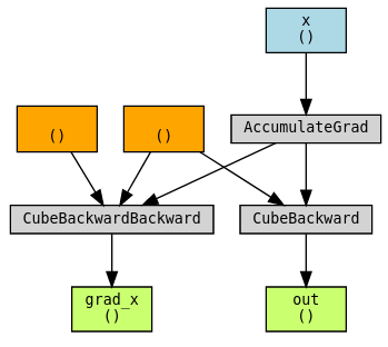
總而言之，自定義函式是否支援雙重反向傳播，取決於反向傳播過程是否可以被 autograd 跟蹤。前兩個示例展示了雙重反向傳播開箱即用的情況。第三個和第四個示例則演示了在通常情況下無法跟蹤反向函式時，如何啟用跟蹤的技術。