對抗樣本生成

建立時間：2018 年 8 月 14 日 | 最後更新：2025 年 1 月 27 日 | 最後驗證：未驗證

作者： Nathan Inkawhich

如果您正在閱讀本文，希望您能理解某些機器學習模型的有效性。研究不斷推動機器學習模型向更快、更準確、更高效的方向發展。然而，設計和訓練模型時一個經常被忽視的方面是安全性與魯棒性，特別是在面對希望欺騙模型的對手時。

本教程將提高您對機器學習模型安全漏洞的認識，並深入瞭解對抗機器學習這一熱門話題。您可能會驚訝地發現，向影像新增幾乎無法察覺的擾動可以導致模型效能出現巨大差異。鑑於這是一個教程，我們將透過影像分類器上的示例來探討該主題。具體來說，我們將使用最早、最受歡迎的攻擊方法之一，快速梯度符號攻擊 (FGSM)，來欺騙 MNIST 分類器。

威脅模型

從背景來看，對抗性攻擊有多種類別，每種類別都有不同的目標和對攻擊者知識的不同假設。然而，總的來說，最終目標是向輸入資料新增最少的擾動，以導致預期的錯誤分類。攻擊者知識的假設有幾種型別，其中兩種是：白盒和黑盒。*白盒*攻擊假設攻擊者對模型有完全的知識和訪問許可權，包括架構、輸入、輸出和權重。*黑盒*攻擊假設攻擊者只能訪問模型的輸入和輸出，對底層架構或權重一無所知。目標也有幾種型別，包括錯誤分類和源/目標錯誤分類。*錯誤分類*的目標意味著對手只希望輸出分類錯誤，而不關心新的分類結果是什麼。*源/目標錯誤分類*意味著對手希望改變一張原本屬於特定源類別的影像，使其被分類為特定的目標類別。

在這種情況下，FGSM 攻擊是一種*白盒*攻擊，目標是*錯誤分類*。有了這些背景資訊，我們現在可以詳細討論這種攻擊了。

快速梯度符號攻擊

迄今為止最早、最受歡迎的對抗攻擊之一被稱為*快速梯度符號攻擊 (FGSM)*，由 Goodfellow 等人在Explaining and Harnessing Adversarial Examples中描述。這種攻擊非常強大，而且直觀。它旨在透過利用神經網路的學習方式（即*梯度*）來攻擊它們。思想很簡單，與其透過根據反向傳播的梯度調整權重來最小化損失，這種攻擊是根據相同的反向傳播梯度*調整輸入資料以最大化損失*。換句話說，這種攻擊使用損失相對於輸入資料的梯度，然後調整輸入資料以最大化損失。

在我們深入程式碼之前，讓我們看看著名的FGSM熊貓示例，並提取一些記號。

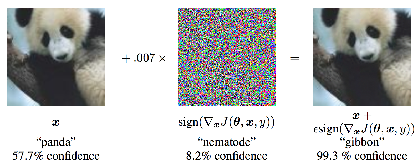
從圖中可知，\(\mathbf{x}\) 是被正確分類為“熊貓”的原始輸入影像，\(y\) 是 \(\mathbf{x}\) 的真實標籤，\(\mathbf{\theta}\) 代表模型引數，\(J(\mathbf{\theta}, \mathbf{x}, y)\) 是用於訓練網路的損失。攻擊將梯度反向傳播到輸入資料以計算 \(\nabla_{x} J(\mathbf{\theta}, \mathbf{x}, y)\)。然後，它透過一個小的步長（圖中為 \(\epsilon\) 或 \(0.007\)）在最大化損失的方向（即 \(sign(\nabla_{x} J(\mathbf{\theta}, \mathbf{x}, y))\)）調整輸入資料。由此產生的擾動影像 \(x'\) 隨後被目標網路*錯誤分類*為“長臂猿”，而它顯然仍然是一隻“熊貓”。

希望現在您已經清楚本教程的動機了，那麼讓我們跳入實現。

import torch
import torch.nn as nn
import torch.nn.functional as F
import torch.optim as optim
from torchvision import datasets, transforms
import numpy as np
import matplotlib.pyplot as plt

實現

在本節中，我們將討論本教程的輸入引數，定義受攻擊的模型，然後編寫攻擊程式碼並執行一些測試。

輸入

本教程只有三個輸入，定義如下

• epsilons - 用於執行的 epsilon 值列表。將 0 包含在列表中很重要，因為它代表模型在原始測試集上的效能。此外，直觀上我們預計 epsilon 越大，擾動越明顯，但在降低模型準確率方面攻擊越有效。由於這裡的資料範圍是 \([0,1]\)，任何 epsilon 值都不應超過 1。

• pretrained_model - 預訓練的 MNIST 模型路徑，該模型使用 pytorch/examples/mnist 訓練。為了簡化，請點選此處下載預訓練模型。

epsilons = [0, .05, .1, .15, .2, .25, .3]
pretrained_model = "data/lenet_mnist_model.pth"
# Set random seed for reproducibility
torch.manual_seed(42)

<torch._C.Generator object at 0x7f5ee6596470>

受攻擊的模型

如前所述，受攻擊的模型與 pytorch/examples/mnist 中的 MNIST 模型相同。您可以自己訓練並儲存 MNIST 模型，也可以下載和使用提供的模型。這裡的 *Net* 定義和測試資料載入器已經從 MNIST 示例中複製。本節的目的是定義模型和資料載入器，然後初始化模型並載入預訓練權重。

# LeNet Model definition
class Net(nn.Module):
    def __init__(self):
        super(Net, self).__init__()
        self.conv1 = nn.Conv2d(1, 32, 3, 1)
        self.conv2 = nn.Conv2d(32, 64, 3, 1)
        self.dropout1 = nn.Dropout(0.25)
        self.dropout2 = nn.Dropout(0.5)
        self.fc1 = nn.Linear(9216, 128)
        self.fc2 = nn.Linear(128, 10)

    def forward(self, x):
        x = self.conv1(x)
        x = F.relu(x)
        x = self.conv2(x)
        x = F.relu(x)
        x = F.max_pool2d(x, 2)
        x = self.dropout1(x)
        x = torch.flatten(x, 1)
        x = self.fc1(x)
        x = F.relu(x)
        x = self.dropout2(x)
        x = self.fc2(x)
        output = F.log_softmax(x, dim=1)
        return output

# MNIST Test dataset and dataloader declaration
test_loader = torch.utils.data.DataLoader(
    datasets.MNIST('../data', train=False, download=True, transform=transforms.Compose([
            transforms.ToTensor(),
            transforms.Normalize((0.1307,), (0.3081,)),
            ])),
        batch_size=1, shuffle=True)

# We want to be able to train our model on an `accelerator <https://pytorch.com.tw/docs/stable/torch.html#accelerators>`__
# such as CUDA, MPS, MTIA, or XPU. If the current accelerator is available, we will use it. Otherwise, we use the CPU.
device = torch.accelerator.current_accelerator().type if torch.accelerator.is_available() else "cpu"
print(f"Using {device} device")

# Initialize the network
model = Net().to(device)

# Load the pretrained model
model.load_state_dict(torch.load(pretrained_model, map_location=device, weights_only=True))

# Set the model in evaluation mode. In this case this is for the Dropout layers
model.eval()

  0%|          | 0.00/9.91M [00:00<?, ?B/s]
100%|##########| 9.91M/9.91M [00:00<00:00, 139MB/s]

  0%|          | 0.00/28.9k [00:00<?, ?B/s]
100%|##########| 28.9k/28.9k [00:00<00:00, 18.2MB/s]

  0%|          | 0.00/1.65M [00:00<?, ?B/s]
100%|##########| 1.65M/1.65M [00:00<00:00, 42.9MB/s]

  0%|          | 0.00/4.54k [00:00<?, ?B/s]
100%|##########| 4.54k/4.54k [00:00<00:00, 30.9MB/s]
Using cuda device

Net(
  (conv1): Conv2d(1, 32, kernel_size=(3, 3), stride=(1, 1))
  (conv2): Conv2d(32, 64, kernel_size=(3, 3), stride=(1, 1))
  (dropout1): Dropout(p=0.25, inplace=False)
  (dropout2): Dropout(p=0.5, inplace=False)
  (fc1): Linear(in_features=9216, out_features=128, bias=True)
  (fc2): Linear(in_features=128, out_features=10, bias=True)
)

FGSM 攻擊

現在，我們可以定義透過擾動原始輸入來建立對抗樣本的函式。fgsm_attack 函式接受三個輸入，image 是原始乾淨影像（\(x\)），epsilon 是畫素級擾動量（\(\epsilon\)），而 data_grad 是損失相對於輸入影像的梯度（\(\nabla_{x} J(\mathbf{\theta}, \mathbf{x}, y)\)）。然後該函式建立擾動影像如下：

\[perturbed\_image = image + epsilon*sign(data\_grad) = x + \epsilon * sign(\nabla_{x} J(\mathbf{\theta}, \mathbf{x}, y)) \]

最後，為了保持資料的原始範圍，擾動影像會被裁剪到 \([0,1]\) 的範圍。

# FGSM attack code
def fgsm_attack(image, epsilon, data_grad):
    # Collect the element-wise sign of the data gradient
    sign_data_grad = data_grad.sign()
    # Create the perturbed image by adjusting each pixel of the input image
    perturbed_image = image + epsilon*sign_data_grad
    # Adding clipping to maintain [0,1] range
    perturbed_image = torch.clamp(perturbed_image, 0, 1)
    # Return the perturbed image
    return perturbed_image

# restores the tensors to their original scale
def denorm(batch, mean=[0.1307], std=[0.3081]):
    """
    Convert a batch of tensors to their original scale.

    Args:
        batch (torch.Tensor): Batch of normalized tensors.
        mean (torch.Tensor or list): Mean used for normalization.
        std (torch.Tensor or list): Standard deviation used for normalization.

    Returns:
        torch.Tensor: batch of tensors without normalization applied to them.
    """
    if isinstance(mean, list):
        mean = torch.tensor(mean).to(device)
    if isinstance(std, list):
        std = torch.tensor(std).to(device)

    return batch * std.view(1, -1, 1, 1) + mean.view(1, -1, 1, 1)

測試函式

最後，本教程的核心結果來自 test 函式。每次呼叫此測試函式都會在 MNIST 測試集上執行完整的測試步驟，並報告最終準確率。然而，請注意，此函式還接受一個 *epsilon* 輸入。這是因為 test 函式報告的是受強度為 \(\epsilon\) 的對手攻擊下的模型準確率。更具體地說，對於測試集中的每個樣本，該函式計算損失相對於輸入資料（\(data\_grad\)）的梯度，使用 fgsm_attack 建立一個擾動影像（\(perturbed\_data\)），然後檢查擾動樣本是否是對抗性的。除了測試模型的準確率外，該函式還會儲存並返回一些成功的對抗樣本，以便稍後進行視覺化。

def test( model, device, test_loader, epsilon ):

    # Accuracy counter
    correct = 0
    adv_examples = []

    # Loop over all examples in test set
    for data, target in test_loader:

        # Send the data and label to the device
        data, target = data.to(device), target.to(device)

        # Set requires_grad attribute of tensor. Important for Attack
        data.requires_grad = True

        # Forward pass the data through the model
        output = model(data)
        init_pred = output.max(1, keepdim=True)[1] # get the index of the max log-probability

        # If the initial prediction is wrong, don't bother attacking, just move on
        if init_pred.item() != target.item():
            continue

        # Calculate the loss
        loss = F.nll_loss(output, target)

        # Zero all existing gradients
        model.zero_grad()

        # Calculate gradients of model in backward pass
        loss.backward()

        # Collect ``datagrad``
        data_grad = data.grad.data

        # Restore the data to its original scale
        data_denorm = denorm(data)

        # Call FGSM Attack
        perturbed_data = fgsm_attack(data_denorm, epsilon, data_grad)

        # Reapply normalization
        perturbed_data_normalized = transforms.Normalize((0.1307,), (0.3081,))(perturbed_data)

        # Re-classify the perturbed image
        output = model(perturbed_data_normalized)

        # Check for success
        final_pred = output.max(1, keepdim=True)[1] # get the index of the max log-probability
        if final_pred.item() == target.item():
            correct += 1
            # Special case for saving 0 epsilon examples
            if epsilon == 0 and len(adv_examples) < 5:
                adv_ex = perturbed_data.squeeze().detach().cpu().numpy()
                adv_examples.append( (init_pred.item(), final_pred.item(), adv_ex) )
        else:
            # Save some adv examples for visualization later
            if len(adv_examples) < 5:
                adv_ex = perturbed_data.squeeze().detach().cpu().numpy()
                adv_examples.append( (init_pred.item(), final_pred.item(), adv_ex) )

    # Calculate final accuracy for this epsilon
    final_acc = correct/float(len(test_loader))
    print(f"Epsilon: {epsilon}\tTest Accuracy = {correct} / {len(test_loader)} = {final_acc}")

    # Return the accuracy and an adversarial example
    return final_acc, adv_examples

執行攻擊

實現的最後一部分是實際執行攻擊。在這裡，我們對 epsilons 輸入中的每個 epsilon 值執行一個完整的測試步驟。對於每個 epsilon，我們還儲存最終準確率和一些成功的對抗樣本，以便在後續章節中進行繪製。請注意，打印出的準確率隨著 epsilon 值的增加而降低。此外，請注意 \(\epsilon=0\) 的情況代表原始測試準確率，沒有任何攻擊。

accuracies = []
examples = []

# Run test for each epsilon
for eps in epsilons:
    acc, ex = test(model, device, test_loader, eps)
    accuracies.append(acc)
    examples.append(ex)

Epsilon: 0      Test Accuracy = 9912 / 10000 = 0.9912
Epsilon: 0.05   Test Accuracy = 9605 / 10000 = 0.9605
Epsilon: 0.1    Test Accuracy = 8743 / 10000 = 0.8743
Epsilon: 0.15   Test Accuracy = 7108 / 10000 = 0.7108
Epsilon: 0.2    Test Accuracy = 4874 / 10000 = 0.4874
Epsilon: 0.25   Test Accuracy = 2710 / 10000 = 0.271
Epsilon: 0.3    Test Accuracy = 1420 / 10000 = 0.142

結果

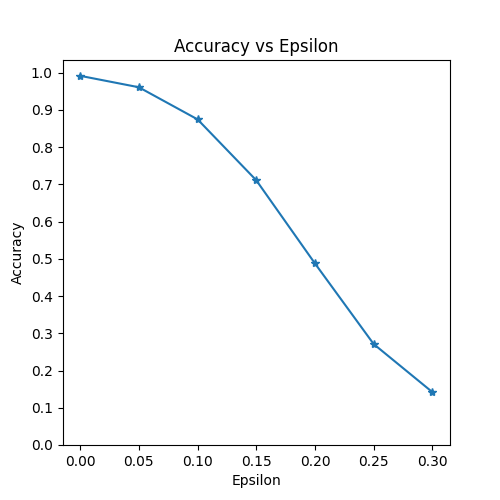
準確率與 Epsilon 的關係

第一個結果是準確率與 epsilon 的關係圖。正如前面提到的，隨著 epsilon 的增加，我們期望測試準確率降低。這是因為更大的 epsilon 意味著我們在最大化損失的方向上邁出了更大的步長。請注意，曲線的趨勢不是線性的，即使 epsilon 值是線性間隔的。例如，\(\epsilon=0.05\) 時的準確率僅比 \(\epsilon=0\) 低約 4%，但 \(\epsilon=0.2\) 時的準確率比 \(\epsilon=0.15\) 低 25%。此外，請注意，對於一個 10 類分類器，模型在 \(\epsilon=0.25\) 和 \(\epsilon=0.3\) 之間達到了隨機猜測的準確率。

plt.figure(figsize=(5,5))
plt.plot(epsilons, accuracies, "*-")
plt.yticks(np.arange(0, 1.1, step=0.1))
plt.xticks(np.arange(0, .35, step=0.05))
plt.title("Accuracy vs Epsilon")
plt.xlabel("Epsilon")
plt.ylabel("Accuracy")
plt.show()

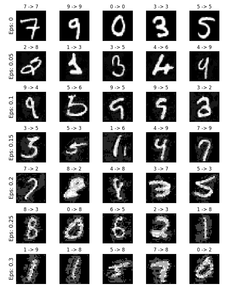
對抗樣本示例

還記得沒有免費午餐的理念嗎？在這種情況下，隨著 epsilon 的增加，測試準確率會下降，但擾動會變得更容易察覺。實際上，準確率下降和可感知性之間存在權衡，攻擊者必須考慮這一點。在這裡，我們展示了一些在每個 epsilon 值下成功的對抗樣本示例。圖的每一行顯示不同的 epsilon 值。第一行是 \(\epsilon=0\) 的示例，代表沒有擾動的原始“乾淨”影像。每個影像的標題顯示“原始分類 -> 對抗分類”。請注意，擾動在 \(\epsilon=0.15\) 時開始變得明顯，在 \(\epsilon=0.3\) 時相當明顯。然而，在所有情況下，儘管添加了噪聲，人類仍然能夠識別出正確的類別。

# Plot several examples of adversarial samples at each epsilon
cnt = 0
plt.figure(figsize=(8,10))
for i in range(len(epsilons)):
    for j in range(len(examples[i])):
        cnt += 1
        plt.subplot(len(epsilons),len(examples[0]),cnt)
        plt.xticks([], [])
        plt.yticks([], [])
        if j == 0:
            plt.ylabel(f"Eps: {epsilons[i]}", fontsize=14)
        orig,adv,ex = examples[i][j]
        plt.title(f"{orig} -> {adv}")
        plt.imshow(ex, cmap="gray")
plt.tight_layout()
plt.show()

下一步做什麼？

希望本教程能讓您對對抗機器學習的主題有所瞭解。接下來有許多潛在的方向。這種攻擊代表了對抗攻擊研究的開端，此後出現了許多關於如何攻擊和防禦來自對手的機器學習模型的想法。實際上，在 NIPS 2017 上有一場對抗攻擊和防禦競賽，競賽中使用的許多方法都在這篇論文中有所描述：Adversarial Attacks and Defences Competition。防禦工作也引出了一個更普遍的理念，即如何使機器學習模型對自然擾動和對抗性精心製作的輸入更具魯棒性。

另一個方向是在不同領域進行對抗攻擊和防禦。對抗性研究不限於影像領域，請檢視這篇針對語音轉文字模型的攻擊。但也許瞭解對抗機器學習的最佳方法是親自動手。嘗試實現一個來自 NIPS 2017 競賽的不同攻擊，看看它與 FGSM 有何不同。然後，嘗試防禦模型免受你自己攻擊。

另一個方向，取決於可用資源，是修改程式碼以支援批次、並行和/或分散式處理，而不是像上面在每個 epsilon test() 迴圈中那樣一次處理一個攻擊。