


注意
點選 此處 下載完整示例程式碼
介紹 || 張量 || Autograd || 構建模型 || TensorBoard 支援 || 訓練模型 || 模型理解
PyTorch TensorBoard 支援
創建於: Nov 30, 2021 | 最後更新: May 29, 2024 | 最後驗證: Nov 05, 2024
請跟隨下面的影片或在 youtube 上觀看。
開始之前
要執行本教程,你需要安裝 PyTorch、TorchVision、Matplotlib 和 TensorBoard。
使用 conda
conda install pytorch torchvision -c pytorch
conda install matplotlib tensorboard
使用 pip
pip install torch torchvision matplotlib tensorboard
安裝完依賴後,請在你安裝它們所在的 Python 環境中重新啟動此 notebook。
引言
在本 notebook 中,我們將針對 Fashion-MNIST 資料集訓練一個 LeNet-5 的變體。Fashion-MNIST 是一組描繪各種服裝的影像塊,帶有十個類別標籤,指示所描繪服裝的型別。
# PyTorch model and training necessities
import torch
import torch.nn as nn
import torch.nn.functional as F
import torch.optim as optim

# Image datasets and image manipulation
import torchvision
import torchvision.transforms as transforms

# Image display
import matplotlib.pyplot as plt
import numpy as np

# PyTorch TensorBoard support
from torch.utils.tensorboard import SummaryWriter

# In case you are using an environment that has TensorFlow installed,
# such as Google Colab, uncomment the following code to avoid
# a bug with saving embeddings to your TensorBoard directory

# import tensorflow as tf
# import tensorboard as tb
# tf.io.gfile = tb.compat.tensorflow_stub.io.gfile
在 TensorBoard 中顯示影像
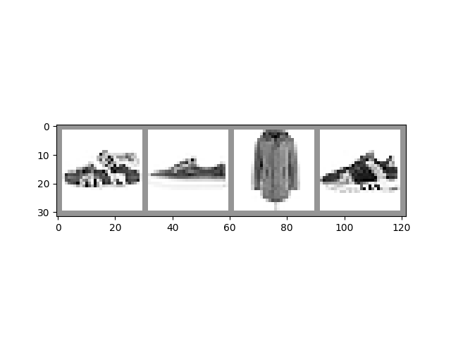
讓我們首先將資料集中的樣本影像新增到 TensorBoard
# Gather datasets and prepare them for consumption
transform = transforms.Compose(
    [transforms.ToTensor(),
    transforms.Normalize((0.5,), (0.5,))])

# Store separate training and validations splits in ./data
training_set = torchvision.datasets.FashionMNIST('./data',
    download=True,
    train=True,
    transform=transform)
validation_set = torchvision.datasets.FashionMNIST('./data',
    download=True,
    train=False,
    transform=transform)

training_loader = torch.utils.data.DataLoader(training_set,
                                              batch_size=4,
                                              shuffle=True,
                                              num_workers=2)


validation_loader = torch.utils.data.DataLoader(validation_set,
                                                batch_size=4,
                                                shuffle=False,
                                                num_workers=2)

# Class labels
classes = ('T-shirt/top', 'Trouser', 'Pullover', 'Dress', 'Coat',
        'Sandal', 'Shirt', 'Sneaker', 'Bag', 'Ankle Boot')

# Helper function for inline image display
def matplotlib_imshow(img, one_channel=False):
    if one_channel:
        img = img.mean(dim=0)
    img = img / 2 + 0.5     # unnormalize
    npimg = img.numpy()
    if one_channel:
        plt.imshow(npimg, cmap="Greys")
    else:
        plt.imshow(np.transpose(npimg, (1, 2, 0)))

# Extract a batch of 4 images
dataiter = iter(training_loader)
images, labels = next(dataiter)

# Create a grid from the images and show them
img_grid = torchvision.utils.make_grid(images)
matplotlib_imshow(img_grid, one_channel=True)
  0%|          | 0.00/26.4M [00:00<?, ?B/s]
  0%|          | 65.5k/26.4M [00:00<01:13, 361kB/s]
  1%|          | 229k/26.4M [00:00<00:37, 692kB/s]
  3%|3         | 918k/26.4M [00:00<00:09, 2.67MB/s]
  7%|7         | 1.93M/26.4M [00:00<00:06, 4.04MB/s]
 26%|##6       | 6.95M/26.4M [00:00<00:01, 13.3MB/s]
 42%|####2     | 11.1M/26.4M [00:00<00:00, 20.0MB/s]
 57%|#####6    | 15.0M/26.4M [00:01<00:00, 24.6MB/s]
 72%|#######2  | 19.0M/26.4M [00:01<00:00, 28.8MB/s]
 85%|########5 | 22.6M/26.4M [00:01<00:00, 27.1MB/s]
 98%|#########7| 25.8M/26.4M [00:01<00:00, 28.4MB/s]
100%|##########| 26.4M/26.4M [00:01<00:00, 19.2MB/s]

  0%|          | 0.00/29.5k [00:00<?, ?B/s]
100%|##########| 29.5k/29.5k [00:00<00:00, 324kB/s]

  0%|          | 0.00/4.42M [00:00<?, ?B/s]
  1%|1         | 65.5k/4.42M [00:00<00:12, 359kB/s]
  5%|5         | 229k/4.42M [00:00<00:06, 675kB/s]
 19%|#9        | 852k/4.42M [00:00<00:01, 2.36MB/s]
 44%|####3     | 1.93M/4.42M [00:00<00:00, 4.11MB/s]
100%|##########| 4.42M/4.42M [00:00<00:00, 6.03MB/s]

  0%|          | 0.00/5.15k [00:00<?, ?B/s]
100%|##########| 5.15k/5.15k [00:00<00:00, 55.5MB/s]
上面,我們使用 TorchVision 和 Matplotlib 建立了輸入資料 minibatch 的可視網格。下面,我們在 SummaryWriter 上使用 add_image() 呼叫,將影像記錄到 TensorBoard 供其使用,並且我們還呼叫 flush() 以確保它立即寫入磁碟。
# Default log_dir argument is "runs" - but it's good to be specific
# torch.utils.tensorboard.SummaryWriter is imported above
writer = SummaryWriter('runs/fashion_mnist_experiment_1')

# Write image data to TensorBoard log dir
writer.add_image('Four Fashion-MNIST Images', img_grid)
writer.flush()

# To view, start TensorBoard on the command line with:
#   tensorboard --logdir=runs
# ...and open a browser tab to https://:6006/
如果你在命令列啟動 TensorBoard 並在新的瀏覽器標籤頁中開啟它(通常在 localhost:6006),你應該在 IMAGES 標籤頁下看到影像網格。
繪製標量以視覺化訓練過程
TensorBoard 對於跟蹤訓練的進度和效果很有用。下面,我們將執行一個訓練迴圈,跟蹤一些指標,並儲存資料供 TensorBoard 使用。
讓我們定義一個模型來對影像塊進行分類,以及一個用於訓練的最佳化器和損失函式
class Net(nn.Module):
    def __init__(self):
        super(Net, self).__init__()
        self.conv1 = nn.Conv2d(1, 6, 5)
        self.pool = nn.MaxPool2d(2, 2)
        self.conv2 = nn.Conv2d(6, 16, 5)
        self.fc1 = nn.Linear(16 * 4 * 4, 120)
        self.fc2 = nn.Linear(120, 84)
        self.fc3 = nn.Linear(84, 10)

    def forward(self, x):
        x = self.pool(F.relu(self.conv1(x)))
        x = self.pool(F.relu(self.conv2(x)))
        x = x.view(-1, 16 * 4 * 4)
        x = F.relu(self.fc1(x))
        x = F.relu(self.fc2(x))
        x = self.fc3(x)
        return x


net = Net()
criterion = nn.CrossEntropyLoss()
optimizer = optim.SGD(net.parameters(), lr=0.001, momentum=0.9)
現在讓我們訓練一個 epoch,並每隔 1000 個 batch 評估訓練集和驗證集的損失
print(len(validation_loader))
for epoch in range(1):  # loop over the dataset multiple times
    running_loss = 0.0

    for i, data in enumerate(training_loader, 0):
        # basic training loop
        inputs, labels = data
        optimizer.zero_grad()
        outputs = net(inputs)
        loss = criterion(outputs, labels)
        loss.backward()
        optimizer.step()

        running_loss += loss.item()
        if i % 1000 == 999:    # Every 1000 mini-batches...
            print('Batch {}'.format(i + 1))
            # Check against the validation set
            running_vloss = 0.0

            # In evaluation mode some model specific operations can be omitted eg. dropout layer
            net.train(False) # Switching to evaluation mode, eg. turning off regularisation
            for j, vdata in enumerate(validation_loader, 0):
                vinputs, vlabels = vdata
                voutputs = net(vinputs)
                vloss = criterion(voutputs, vlabels)
                running_vloss += vloss.item()
            net.train(True) # Switching back to training mode, eg. turning on regularisation

            avg_loss = running_loss / 1000
            avg_vloss = running_vloss / len(validation_loader)

            # Log the running loss averaged per batch
            writer.add_scalars('Training vs. Validation Loss',
                            { 'Training' : avg_loss, 'Validation' : avg_vloss },
                            epoch * len(training_loader) + i)

            running_loss = 0.0
print('Finished Training')

writer.flush()
2500
Batch 1000
Batch 2000
Batch 3000
Batch 4000
Batch 5000
Batch 6000
Batch 7000
Batch 8000
Batch 9000
Batch 10000
Batch 11000
Batch 12000
Batch 13000
Batch 14000
Batch 15000
Finished Training
切換到你已開啟的 TensorBoard,檢視 SCALARS 標籤頁。
視覺化你的模型
TensorBoard 也可用於檢查模型內的資料流。為此,請使用模型和樣本輸入呼叫 add_graph() 方法
# Again, grab a single mini-batch of images
dataiter = iter(training_loader)
images, labels = next(dataiter)

# add_graph() will trace the sample input through your model,
# and render it as a graph.
writer.add_graph(net, images)
writer.flush()
當你切換到 TensorBoard 時,你應該會看到一個 GRAPHS 標籤頁。雙擊“NET”節點以檢視模型內的層和資料流。
使用嵌入視覺化你的資料集
我們使用的 28x28 影像塊可以建模為 784 維向量 (28 * 28 = 784)。將其投影到低維表示是有益的。add_embedding() 方法會將一組資料投影到方差最高的三個維度上,並將其顯示為互動式 3D 圖表。add_embedding() 方法透過投影到方差最高的三個維度來自動完成此操作。
下面,我們將抽取一部分資料,並生成這樣的嵌入
# Select a random subset of data and corresponding labels
def select_n_random(data, labels, n=100):
    assert len(data) == len(labels)

    perm = torch.randperm(len(data))
    return data[perm][:n], labels[perm][:n]

# Extract a random subset of data
images, labels = select_n_random(training_set.data, training_set.targets)

# get the class labels for each image
class_labels = [classes[label] for label in labels]

# log embeddings
features = images.view(-1, 28 * 28)
writer.add_embedding(features,
                    metadata=class_labels,
                    label_img=images.unsqueeze(1))
writer.flush()
writer.close()
現在,如果你切換到 TensorBoard 並選擇 PROJECTOR 標籤頁,你應該會看到投影的 3D 表示。你可以旋轉和縮放模型。在大尺度和小尺度下檢查它,看看能否發現投影資料中的模式和標籤的聚類。
為了獲得更好的視覺化效果,建議
在左側的“Color by”下拉選單中選擇“label”。
切換頂部的夜間模式圖示,將淺色影像放在深色背景上。
其他資源
欲瞭解更多資訊,請參閱
關於
torch.utils.tensorboard.SummaryWriter的 PyTorch 文件PyTorch.org 教程 的 Tensorboard 教程內容
欲瞭解更多關於 TensorBoard 的資訊,請參閱 TensorBoard 文件
指令碼總執行時間: ( 1 分 51.246 秒)
