


注意
點選此處下載完整的示例程式碼
訓練分類器
創建於: 2017 年 3 月 24 日 | 最後更新於: 2024 年 12 月 20 日 | 最後驗證於: 未驗證
就是這樣。您已經瞭解瞭如何定義神經網路、計算損失以及更新網路權重。
現在您可能會想,
資料怎麼辦?
通常,當您需要處理影像、文字、音訊或影片資料時,可以使用標準的 Python 包將資料載入到 numpy 陣列中。然後,您可以將此陣列轉換為 torch.*Tensor。
對於影像,Pillow、OpenCV 等包很有用
對於音訊,scipy 和 librosa 等包很有用
對於文字,可以使用原生 Python 或基於 Cython 的載入方式,或者使用 NLTK 和 SpaCy 等包
特別是在視覺領域,我們建立了一個名為 torchvision 的包,它包含了 ImageNet、CIFAR10、MNIST 等常見資料集的資料載入器,以及影像資料轉換器,即 torchvision.datasets 和 torch.utils.data.DataLoader。
這提供了極大的便利,避免編寫樣板程式碼。
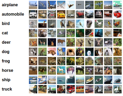
在本教程中,我們將使用 CIFAR10 資料集。它包含以下類別:‘airplane’(飛機)、‘automobile’(汽車)、‘bird’(鳥)、‘cat’(貓)、‘deer’(鹿)、‘dog’(狗)、‘frog’(青蛙)、‘horse’(馬)、‘ship’(船)、‘truck’(卡車)。CIFAR-10 中的影像大小為 3x32x32,即大小為 32x32 畫素的 3 通道彩色影像。
cifar10
訓練影像分類器
我們將按以下步驟進行
使用
torchvision載入並歸一化 CIFAR10 訓練集和測試集定義一個卷積神經網路
定義一個損失函式
在訓練資料上訓練網路
在測試資料上測試網路
1. 載入並歸一化 CIFAR10
使用 torchvision 載入 CIFAR10 非常容易。
import torch
import torchvision
import torchvision.transforms as transforms
torchvision 資料集的輸出是範圍在 [0, 1] 的 PILImage 影像。我們將它們轉換為範圍在 [-1, 1] 的歸一化張量。
注意
如果在 Windows 上執行並出現 BrokenPipeError,請嘗試將 torch.utils.data.DataLoader() 的 num_worker 設定為 0。
transform = transforms.Compose(
    [transforms.ToTensor(),
     transforms.Normalize((0.5, 0.5, 0.5), (0.5, 0.5, 0.5))])

batch_size = 4

trainset = torchvision.datasets.CIFAR10(root='./data', train=True,
                                        download=True, transform=transform)
trainloader = torch.utils.data.DataLoader(trainset, batch_size=batch_size,
                                          shuffle=True, num_workers=2)

testset = torchvision.datasets.CIFAR10(root='./data', train=False,
                                       download=True, transform=transform)
testloader = torch.utils.data.DataLoader(testset, batch_size=batch_size,
                                         shuffle=False, num_workers=2)

classes = ('plane', 'car', 'bird', 'cat',
           'deer', 'dog', 'frog', 'horse', 'ship', 'truck')
  0%|          | 0.00/170M [00:00<?, ?B/s]
  0%|          | 459k/170M [00:00<00:37, 4.58MB/s]
  4%|4         | 7.63M/170M [00:00<00:03, 44.1MB/s]
 11%|#         | 18.3M/170M [00:00<00:02, 72.2MB/s]
 17%|#6        | 28.5M/170M [00:00<00:01, 83.9MB/s]
 23%|##2       | 39.2M/170M [00:00<00:01, 92.1MB/s]
 29%|##9       | 49.7M/170M [00:00<00:01, 96.5MB/s]
 36%|###5      | 60.6M/170M [00:00<00:01, 101MB/s]
 42%|####1     | 70.8M/170M [00:00<00:00, 101MB/s]
 48%|####7     | 81.4M/170M [00:00<00:00, 103MB/s]
 54%|#####3    | 91.8M/170M [00:01<00:00, 103MB/s]
 60%|######    | 103M/170M [00:01<00:00, 104MB/s]
 67%|######6   | 114M/170M [00:01<00:00, 106MB/s]
 73%|#######2  | 124M/170M [00:01<00:00, 106MB/s]
 79%|#######9  | 135M/170M [00:01<00:00, 107MB/s]
 86%|########5 | 146M/170M [00:01<00:00, 105MB/s]
 92%|#########1| 157M/170M [00:01<00:00, 105MB/s]
 98%|#########8| 167M/170M [00:01<00:00, 104MB/s]
100%|##########| 170M/170M [00:01<00:00, 97.7MB/s]
讓我們展示一些訓練影像,以供參考。
import matplotlib.pyplot as plt
import numpy as np

# functions to show an image


def imshow(img):
    img = img / 2 + 0.5     # unnormalize
    npimg = img.numpy()
    plt.imshow(np.transpose(npimg, (1, 2, 0)))
    plt.show()


# get some random training images
dataiter = iter(trainloader)
images, labels = next(dataiter)

# show images
imshow(torchvision.utils.make_grid(images))
# print labels
print(' '.join(f'{classes[labels[j]]:5s}' for j in range(batch_size)))
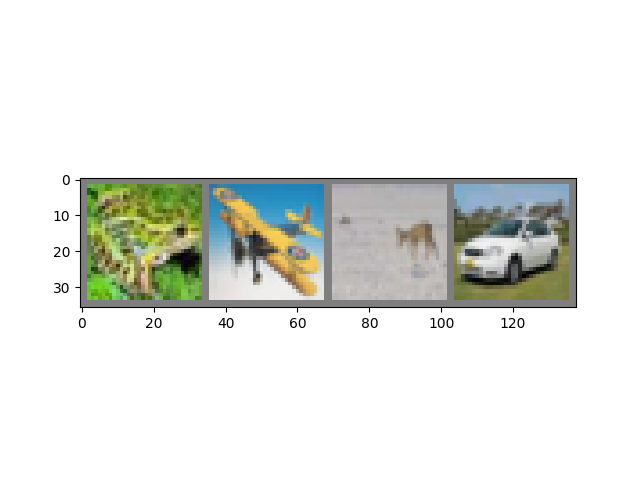
frog plane deer car
2. 定義一個卷積神經網路
複製前面“神經網路”部分中的神經網路,並修改它以接收 3 通道影像(而不是之前定義的 1 通道影像)。
import torch.nn as nn
import torch.nn.functional as F


class Net(nn.Module):
    def __init__(self):
        super().__init__()
        self.conv1 = nn.Conv2d(3, 6, 5)
        self.pool = nn.MaxPool2d(2, 2)
        self.conv2 = nn.Conv2d(6, 16, 5)
        self.fc1 = nn.Linear(16 * 5 * 5, 120)
        self.fc2 = nn.Linear(120, 84)
        self.fc3 = nn.Linear(84, 10)

    def forward(self, x):
        x = self.pool(F.relu(self.conv1(x)))
        x = self.pool(F.relu(self.conv2(x)))
        x = torch.flatten(x, 1) # flatten all dimensions except batch
        x = F.relu(self.fc1(x))
        x = F.relu(self.fc2(x))
        x = self.fc3(x)
        return x


net = Net()
3. 定義損失函式和最佳化器
讓我們使用分類交叉熵損失和帶動量的 SGD。
import torch.optim as optim

criterion = nn.CrossEntropyLoss()
optimizer = optim.SGD(net.parameters(), lr=0.001, momentum=0.9)
4. 訓練網路
這時候事情開始變得有趣了。我們只需遍歷資料迭代器,將輸入饋送到網路並進行最佳化。
for epoch in range(2):  # loop over the dataset multiple times

    running_loss = 0.0
    for i, data in enumerate(trainloader, 0):
        # get the inputs; data is a list of [inputs, labels]
        inputs, labels = data

        # zero the parameter gradients
        optimizer.zero_grad()

        # forward + backward + optimize
        outputs = net(inputs)
        loss = criterion(outputs, labels)
        loss.backward()
        optimizer.step()

        # print statistics
        running_loss += loss.item()
        if i % 2000 == 1999:    # print every 2000 mini-batches
            print(f'[{epoch + 1}, {i + 1:5d}] loss: {running_loss / 2000:.3f}')
            running_loss = 0.0

print('Finished Training')
[1,  2000] loss: 2.143
[1,  4000] loss: 1.833
[1,  6000] loss: 1.674
[1,  8000] loss: 1.574
[1, 10000] loss: 1.524
[1, 12000] loss: 1.445
[2,  2000] loss: 1.405
[2,  4000] loss: 1.363
[2,  6000] loss: 1.339
[2,  8000] loss: 1.342
[2, 10000] loss: 1.311
[2, 12000] loss: 1.274
Finished Training
讓我們快速儲存訓練好的模型
PATH = './cifar_net.pth'
torch.save(net.state_dict(), PATH)
有關儲存 PyTorch 模型的更多詳細資訊,請參閱此處。
5. 在測試資料上測試網路
我們已經對訓練資料集進行了 2 次完整的訓練。但我們需要檢查網路是否學到了任何東西。
我們將透過預測神經網路輸出的類別標籤,並與真實標籤進行對比來檢查。如果預測正確,我們將樣本新增到正確預測列表中。
好的,第一步。讓我們顯示測試集中的一張影像以熟悉情況。
dataiter = iter(testloader)
images, labels = next(dataiter)

# print images
imshow(torchvision.utils.make_grid(images))
print('GroundTruth: ', ' '.join(f'{classes[labels[j]]:5s}' for j in range(4)))
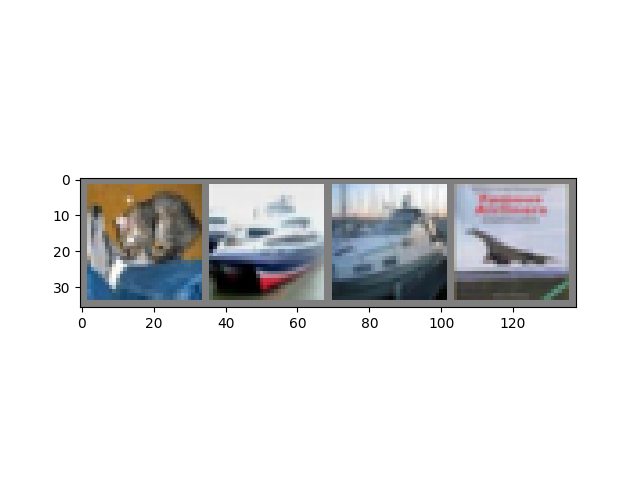
GroundTruth: cat ship ship plane
接下來,讓我們重新載入我們儲存的模型(注意:此處並非必須儲存和重新載入模型,我們只是為了說明如何操作)。
net = Net()
net.load_state_dict(torch.load(PATH, weights_only=True))
<All keys matched successfully>
好的,現在讓我們看看神經網路認為上面的這些示例是什麼
輸出是 10 個類別的“能量”。某個類別的能量越高,網路越認為影像屬於該類別。因此,讓我們獲取能量最高的索引
Predicted: frog ship ship plane
結果看起來相當不錯。
讓我們看看網路在整個資料集上的表現。
correct = 0
total = 0
# since we're not training, we don't need to calculate the gradients for our outputs
with torch.no_grad():
    for data in testloader:
        images, labels = data
        # calculate outputs by running images through the network
        outputs = net(images)
        # the class with the highest energy is what we choose as prediction
        _, predicted = torch.max(outputs, 1)
        total += labels.size(0)
        correct += (predicted == labels).sum().item()

print(f'Accuracy of the network on the 10000 test images: {100 * correct // total} %')
Accuracy of the network on the 10000 test images: 55 %
這看起來比隨機猜測(10 個類別中隨機選擇一個,準確率為 10%)好得多。看來網路學到了一些東西。
嗯,哪些類別的表現很好,哪些類別的表現不好呢?
# prepare to count predictions for each class
correct_pred = {classname: 0 for classname in classes}
total_pred = {classname: 0 for classname in classes}

# again no gradients needed
with torch.no_grad():
    for data in testloader:
        images, labels = data
        outputs = net(images)
        _, predictions = torch.max(outputs, 1)
        # collect the correct predictions for each class
        for label, prediction in zip(labels, predictions):
            if label == prediction:
                correct_pred[classes[label]] += 1
            total_pred[classes[label]] += 1


# print accuracy for each class
for classname, correct_count in correct_pred.items():
    accuracy = 100 * float(correct_count) / total_pred[classname]
    print(f'Accuracy for class: {classname:5s} is {accuracy:.1f} %')
Accuracy for class: plane is 43.5 %
Accuracy for class: car   is 67.2 %
Accuracy for class: bird  is 44.7 %
Accuracy for class: cat   is 29.5 %
Accuracy for class: deer  is 48.9 %
Accuracy for class: dog   is 47.0 %
Accuracy for class: frog  is 60.5 %
Accuracy for class: horse is 70.9 %
Accuracy for class: ship  is 79.8 %
Accuracy for class: truck is 65.4 %
好的,接下來該怎麼辦?
我們如何在 GPU 上執行這些神經網路?
在 GPU 上訓練
就像將張量轉移到 GPU 上一樣,您也需要將神經網路轉移到 GPU 上。
如果我們有 CUDA 可用,讓我們首先將裝置定義為第一個可見的 cuda 裝置
device = torch.device('cuda:0' if torch.cuda.is_available() else 'cpu')

# Assuming that we are on a CUDA machine, this should print a CUDA device:

print(device)
cuda:0
本節的其餘部分假設 device 是一個 CUDA 裝置。
然後這些方法將遞迴地遍歷所有模組,並將它們的引數和緩衝區轉換為 CUDA 張量
net.to(device)
記住,您還需要在每一步將輸入和目標傳送到 GPU
為什麼我沒有注意到與 CPU 相比有巨大的加速?因為您的網路很小。
練習:嘗試增加網路的寬度(第一個 nn.Conv2d 的引數 2 和第二個 nn.Conv2d 的引數 1 – 它們需要是相同的數字),看看能獲得什麼樣的加速。
目標達成:
高度理解 PyTorch 的張量庫和神經網路。
訓練一個小型神經網路對影像進行分類
