注意

點選此處下載完整的示例程式碼

從零開始學自然語言處理：使用字元級 RNN 對名字進行分類¶

建立日期: 2017 年 3 月 24 日 | 最後更新: 2025 年 3 月 14 日 | 最後驗證: 2024 年 11 月 5 日

本教程是一個三部分系列的一部分

我們將構建並訓練一個基本的字元級迴圈神經網路 (RNN) 來對單詞進行分類。本教程與另外兩個“從零開始”的自然語言處理 (NLP) 教程從零開始學自然語言處理：使用字元級 RNN 生成名字和從零開始學自然語言處理：使用序列到序列網路和注意力機制進行翻譯一起，展示瞭如何預處理資料以建模 NLP。特別是，這些教程展示瞭如何以低層次處理資料來建模 NLP。

字元級 RNN 將單詞讀取為一系列字元 - 在每個步驟輸出一個預測和“隱藏狀態”，並將其先前的隱藏狀態饋送到下一個步驟中。我們將最終預測作為輸出，即單詞所屬的類別。

具體來說，我們將訓練資料集包含來自 18 種語言的數千個姓氏，並根據拼寫預測名字來自哪種語言。

準備 Torch¶

設定 torch，使其預設使用正確的裝置，並根據您的硬體（CPU 或 CUDA）使用 GPU 加速。

import torch

# Check if CUDA is available
device = torch.device('cpu')
if torch.cuda.is_available():
    device = torch.device('cuda')

torch.set_default_device(device)
print(f"Using device = {torch.get_default_device()}")

Using device = cuda:0

準備資料¶

從此處下載資料並將其解壓到當前目錄。

data/names 目錄中包含 18 個文字檔案，檔名格式為 [Language].txt。每個檔案包含許多名字，每行一個，大部分已羅馬化（但我們仍然需要從 Unicode 轉換為 ASCII）。

第一步是定義和清理我們的資料。首先，我們需要將 Unicode 轉換為純 ASCII 以限制 RNN 輸入層。這透過將 Unicode 字串轉換為 ASCII 並只允許一小部分允許的字元來實現。

import string
import unicodedata

# We can use "_" to represent an out-of-vocabulary character, that is, any character we are not handling in our model
allowed_characters = string.ascii_letters + " .,;'" + "_"
n_letters = len(allowed_characters)

# Turn a Unicode string to plain ASCII, thanks to https://stackoverflow.com/a/518232/2809427
def unicodeToAscii(s):
    return ''.join(
        c for c in unicodedata.normalize('NFD', s)
        if unicodedata.category(c) != 'Mn'
        and c in allowed_characters
    )

這是一個將 Unicode 字母名字轉換為純 ASCII 的示例。這簡化了輸入層

print (f"converting 'Ślusàrski' to {unicodeToAscii('Ślusàrski')}")

converting 'Ślusàrski' to Slusarski

將名字轉換為張量（Tensors）¶

現在我們已經組織好所有名字，我們需要將它們轉換為張量才能使用它們。

為了表示單個字母，我們使用大小為 <1 x n_letters> 的“one-hot 向量”。one-hot 向量除了當前字母索引處為 1 外，其餘均為 0，例如 "b" = <0 1 0 0 0 ...>。

為了構成一個單詞，我們將這些向量連線成一個 2D 矩陣 <line_length x 1 x n_letters>。

額外的維度 1 是因為 PyTorch 假定所有內容都是批次的 - 我們這裡僅使用批次大小為 1。

# Find letter index from all_letters, e.g. "a" = 0
def letterToIndex(letter):
    # return our out-of-vocabulary character if we encounter a letter unknown to our model
    if letter not in allowed_characters:
        return allowed_characters.find("_")
    else:
        return allowed_characters.find(letter)

# Turn a line into a <line_length x 1 x n_letters>,
# or an array of one-hot letter vectors
def lineToTensor(line):
    tensor = torch.zeros(len(line), 1, n_letters)
    for li, letter in enumerate(line):
        tensor[li][0][letterToIndex(letter)] = 1
    return tensor

這裡有一些如何對單個字元或多個字元字串使用 lineToTensor() 的示例。

print (f"The letter 'a' becomes {lineToTensor('a')}") #notice that the first position in the tensor = 1
print (f"The name 'Ahn' becomes {lineToTensor('Ahn')}") #notice 'A' sets the 27th index to 1

The letter 'a' becomes tensor([[[1., 0., 0., 0., 0., 0., 0., 0., 0., 0., 0., 0., 0., 0., 0., 0., 0.,
          0., 0., 0., 0., 0., 0., 0., 0., 0., 0., 0., 0., 0., 0., 0., 0., 0.,
          0., 0., 0., 0., 0., 0., 0., 0., 0., 0., 0., 0., 0., 0., 0., 0., 0.,
          0., 0., 0., 0., 0., 0., 0.]]], device='cuda:0')
The name 'Ahn' becomes tensor([[[0., 0., 0., 0., 0., 0., 0., 0., 0., 0., 0., 0., 0., 0., 0., 0., 0.,
          0., 0., 0., 0., 0., 0., 0., 0., 0., 1., 0., 0., 0., 0., 0., 0., 0.,
          0., 0., 0., 0., 0., 0., 0., 0., 0., 0., 0., 0., 0., 0., 0., 0., 0.,
          0., 0., 0., 0., 0., 0., 0.]],

        [[0., 0., 0., 0., 0., 0., 0., 1., 0., 0., 0., 0., 0., 0., 0., 0., 0.,
          0., 0., 0., 0., 0., 0., 0., 0., 0., 0., 0., 0., 0., 0., 0., 0., 0.,
          0., 0., 0., 0., 0., 0., 0., 0., 0., 0., 0., 0., 0., 0., 0., 0., 0.,
          0., 0., 0., 0., 0., 0., 0.]],

        [[0., 0., 0., 0., 0., 0., 0., 0., 0., 0., 0., 0., 0., 1., 0., 0., 0.,
          0., 0., 0., 0., 0., 0., 0., 0., 0., 0., 0., 0., 0., 0., 0., 0., 0.,
          0., 0., 0., 0., 0., 0., 0., 0., 0., 0., 0., 0., 0., 0., 0., 0., 0.,
          0., 0., 0., 0., 0., 0., 0.]]], device='cuda:0')

恭喜您，您已經為這項學習任務構建了基礎張量物件！您可以使用類似的方法處理其他文字相關的 RNN 任務。

接下來，我們需要將所有示例組合成一個數據集，以便我們可以訓練、測試和驗證我們的模型。為此，我們將使用 Dataset and DataLoader 類來儲存我們的資料集。每個 Dataset 需要實現三個函式：__init__、__len__ 和 __getitem__。

from io import open
import glob
import os
import time

import torch
from torch.utils.data import Dataset

class NamesDataset(Dataset):

    def __init__(self, data_dir):
        self.data_dir = data_dir #for provenance of the dataset
        self.load_time = time.localtime #for provenance of the dataset
        labels_set = set() #set of all classes

        self.data = []
        self.data_tensors = []
        self.labels = []
        self.labels_tensors = []

        #read all the ``.txt`` files in the specified directory
        text_files = glob.glob(os.path.join(data_dir, '*.txt'))
        for filename in text_files:
            label = os.path.splitext(os.path.basename(filename))[0]
            labels_set.add(label)
            lines = open(filename, encoding='utf-8').read().strip().split('\n')
            for name in lines:
                self.data.append(name)
                self.data_tensors.append(lineToTensor(name))
                self.labels.append(label)

        #Cache the tensor representation of the labels
        self.labels_uniq = list(labels_set)
        for idx in range(len(self.labels)):
            temp_tensor = torch.tensor([self.labels_uniq.index(self.labels[idx])], dtype=torch.long)
            self.labels_tensors.append(temp_tensor)

    def __len__(self):
        return len(self.data)

    def __getitem__(self, idx):
        data_item = self.data[idx]
        data_label = self.labels[idx]
        data_tensor = self.data_tensors[idx]
        label_tensor = self.labels_tensors[idx]

        return label_tensor, data_tensor, data_label, data_item

在這裡，我們可以將示例資料載入到 NamesDataset 中

alldata = NamesDataset("data/names")
print(f"loaded {len(alldata)} items of data")
print(f"example = {alldata[0]}")

loaded 20074 items of data
example = (tensor([2], device='cuda:0'), tensor([[[0., 0., 0., 0., 0., 0., 0., 0., 0., 0., 0., 0., 0., 0., 0., 0., 0.,
          0., 0., 0., 0., 0., 0., 0., 0., 0., 0., 0., 0., 0., 0., 0., 0., 0.,
          0., 0., 1., 0., 0., 0., 0., 0., 0., 0., 0., 0., 0., 0., 0., 0., 0.,
          0., 0., 0., 0., 0., 0., 0.]],

        [[0., 0., 0., 0., 0., 0., 0., 1., 0., 0., 0., 0., 0., 0., 0., 0., 0.,
          0., 0., 0., 0., 0., 0., 0., 0., 0., 0., 0., 0., 0., 0., 0., 0., 0.,
          0., 0., 0., 0., 0., 0., 0., 0., 0., 0., 0., 0., 0., 0., 0., 0., 0.,
          0., 0., 0., 0., 0., 0., 0.]],

        [[0., 0., 0., 0., 0., 0., 0., 0., 0., 0., 0., 0., 0., 0., 1., 0., 0.,
          0., 0., 0., 0., 0., 0., 0., 0., 0., 0., 0., 0., 0., 0., 0., 0., 0.,
          0., 0., 0., 0., 0., 0., 0., 0., 0., 0., 0., 0., 0., 0., 0., 0., 0.,
          0., 0., 0., 0., 0., 0., 0.]],

        [[0., 0., 0., 0., 0., 0., 0., 0., 0., 0., 0., 0., 0., 0., 0., 0., 0.,
          0., 0., 0., 1., 0., 0., 0., 0., 0., 0., 0., 0., 0., 0., 0., 0., 0.,
          0., 0., 0., 0., 0., 0., 0., 0., 0., 0., 0., 0., 0., 0., 0., 0., 0.,
          0., 0., 0., 0., 0., 0., 0.]],

        [[0., 0., 0., 0., 0., 0., 0., 0., 0., 0., 0., 0., 0., 0., 0., 0., 0.,
          1., 0., 0., 0., 0., 0., 0., 0., 0., 0., 0., 0., 0., 0., 0., 0., 0.,
          0., 0., 0., 0., 0., 0., 0., 0., 0., 0., 0., 0., 0., 0., 0., 0., 0.,
          0., 0., 0., 0., 0., 0., 0.]],

        [[0., 0., 0., 0., 0., 0., 0., 0., 0., 0., 0., 0., 0., 0., 0., 0., 0.,
          0., 0., 0., 0., 0., 0., 0., 1., 0., 0., 0., 0., 0., 0., 0., 0., 0.,
          0., 0., 0., 0., 0., 0., 0., 0., 0., 0., 0., 0., 0., 0., 0., 0., 0.,
          0., 0., 0., 0., 0., 0., 0.]]], device='cuda:0'), 'Arabic', 'Khoury')

使用資料集物件，我們可以輕鬆地將資料分成訓練集和測試集。這裡我們建立了一個 80/20: 分割，但 torch.utils.data 提供了更多有用的工具。這裡我們指定一個生成器，因為我們需要使用與 PyTorch 上面預設的裝置相同的裝置。

上面預設的裝置。

train_set, test_set = torch.utils.data.random_split(alldata, [.85, .15], generator=torch.Generator(device=device).manual_seed(2024))

print(f"train examples = {len(train_set)}, validation examples = {len(test_set)}")

train examples = 17063, validation examples = 3011

現在我們擁有一個包含 20074 個示例的基礎資料集，其中每個示例都是標籤和名字的配對。我們還將資料集分成了訓練集和測試集，以便我們可以驗證構建的模型。

建立網路¶

在使用 autograd 之前，在 Torch 中建立迴圈神經網路需要將層的引數在多個時間步上進行克隆。這些層持有隱藏狀態和梯度，現在這些都完全由圖本身處理。這意味著您可以以非常“純粹”的方式實現 RNN，就像常規的前饋層一樣。

此 CharRNN 類實現了具有三個元件的 RNN。首先，我們使用 nn.RNN 實現。接下來，我們定義一個將 RNN 隱藏層對映到我們輸出的層。最後，我們應用一個 softmax 函式。使用 nn.RNN 帶來了顯著的效能提升，例如 cuDNN 加速的核心，而如果將每個層實現為 nn.Linear 則不然。這也簡化了 forward() 中的實現。

import torch.nn as nn
import torch.nn.functional as F

class CharRNN(nn.Module):
    def __init__(self, input_size, hidden_size, output_size):
        super(CharRNN, self).__init__()

        self.rnn = nn.RNN(input_size, hidden_size)
        self.h2o = nn.Linear(hidden_size, output_size)
        self.softmax = nn.LogSoftmax(dim=1)

    def forward(self, line_tensor):
        rnn_out, hidden = self.rnn(line_tensor)
        output = self.h2o(hidden[0])
        output = self.softmax(output)

        return output

然後我們可以建立一個具有 58 個輸入節點、128 個隱藏節點和 18 個輸出的 RNN

n_hidden = 128
rnn = CharRNN(n_letters, n_hidden, len(alldata.labels_uniq))
print(rnn)

CharRNN(
  (rnn): RNN(58, 128)
  (h2o): Linear(in_features=128, out_features=18, bias=True)
  (softmax): LogSoftmax(dim=1)
)

之後，我們可以將張量傳遞給 RNN 以獲得預測輸出。隨後，我們使用輔助函式 label_from_output 來匯出類別的文字標籤。

def label_from_output(output, output_labels):
    top_n, top_i = output.topk(1)
    label_i = top_i[0].item()
    return output_labels[label_i], label_i

input = lineToTensor('Albert')
output = rnn(input) #this is equivalent to ``output = rnn.forward(input)``
print(output)
print(label_from_output(output, alldata.labels_uniq))

tensor([[-2.8627, -2.8503, -2.8578, -3.0326, -2.8298, -2.8469, -2.9527, -2.9330,
         -2.9295, -2.9728, -2.8209, -2.7876, -2.9343, -2.9412, -2.8902, -2.9107,
         -2.8262, -2.8812]], device='cuda:0', grad_fn=<LogSoftmaxBackward0>)
('Italian', 11)

訓練¶

訓練網路¶

現在訓練這個網路所需要做的就是向它展示大量示例，讓它進行猜測，然後告訴它是否猜錯了。

我們透過定義一個 train() 函式來實現這一點，該函式使用小批次對給定資料集進行訓練。RNN 的訓練方式與其他網路類似；因此，為了完整性，這裡包含了一個批次訓練方法。迴圈 (for i in batch) 計算批次中每個專案的損失，然後調整權重。此操作重複進行，直到達到指定的 epoch 數。

import random
import numpy as np

def train(rnn, training_data, n_epoch = 10, n_batch_size = 64, report_every = 50, learning_rate = 0.2, criterion = nn.NLLLoss()):
    """
    Learn on a batch of training_data for a specified number of iterations and reporting thresholds
    """
    # Keep track of losses for plotting
    current_loss = 0
    all_losses = []
    rnn.train()
    optimizer = torch.optim.SGD(rnn.parameters(), lr=learning_rate)

    start = time.time()
    print(f"training on data set with n = {len(training_data)}")

    for iter in range(1, n_epoch + 1):
        rnn.zero_grad() # clear the gradients

        # create some minibatches
        # we cannot use dataloaders because each of our names is a different length
        batches = list(range(len(training_data)))
        random.shuffle(batches)
        batches = np.array_split(batches, len(batches) //n_batch_size )

        for idx, batch in enumerate(batches):
            batch_loss = 0
            for i in batch: #for each example in this batch
                (label_tensor, text_tensor, label, text) = training_data[i]
                output = rnn.forward(text_tensor)
                loss = criterion(output, label_tensor)
                batch_loss += loss

            # optimize parameters
            batch_loss.backward()
            nn.utils.clip_grad_norm_(rnn.parameters(), 3)
            optimizer.step()
            optimizer.zero_grad()

            current_loss += batch_loss.item() / len(batch)

        all_losses.append(current_loss / len(batches) )
        if iter % report_every == 0:
            print(f"{iter} ({iter / n_epoch:.0%}): \t average batch loss = {all_losses[-1]}")
        current_loss = 0

    return all_losses

現在我們可以使用小批次訓練資料集，指定 epoch 數。為了加快構建速度，此示例的 epoch 數已減少。使用不同的引數可以獲得更好的結果。

start = time.time()
all_losses = train(rnn, train_set, n_epoch=27, learning_rate=0.15, report_every=5)
end = time.time()
print(f"training took {end-start}s")

training on data set with n = 17063
(19%):         average batch loss = 0.879241389256809
(37%):        average batch loss = 0.6880160899297428
(56%):        average batch loss = 0.5751259022999389
(74%):        average batch loss = 0.49494854703054325
(93%):        average batch loss = 0.4307829880331761
training took 340.6842153072357s

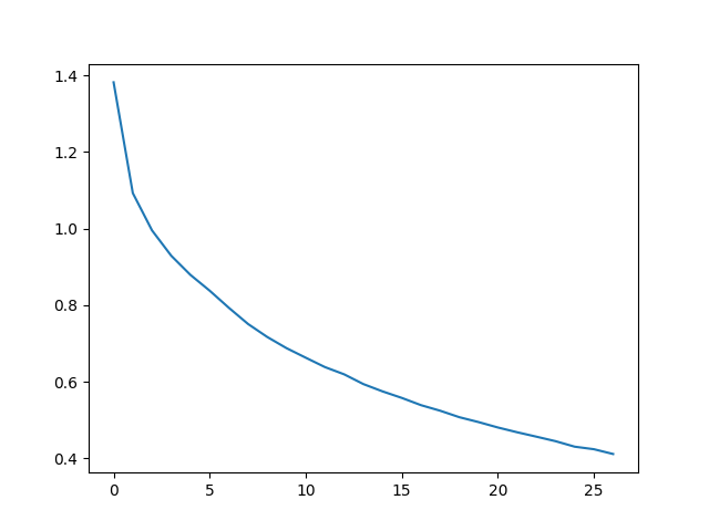
繪製結果¶

繪製來自 all_losses 的歷史損失曲線可以顯示網路的學習情況

import matplotlib.pyplot as plt
import matplotlib.ticker as ticker

plt.figure()
plt.plot(all_losses)
plt.show()

評估結果¶

為了瞭解網路在不同類別上的表現，我們將建立一個混淆矩陣（confusion matrix），顯示對於每個實際語言（行），網路預測的語言（列）。要計算混淆矩陣，需要透過 evaluate() 執行大量樣本，evaluate() 與 train() 相同，只是沒有反向傳播。

def evaluate(rnn, testing_data, classes):
    confusion = torch.zeros(len(classes), len(classes))

    rnn.eval() #set to eval mode
    with torch.no_grad(): # do not record the gradients during eval phase
        for i in range(len(testing_data)):
            (label_tensor, text_tensor, label, text) = testing_data[i]
            output = rnn(text_tensor)
            guess, guess_i = label_from_output(output, classes)
            label_i = classes.index(label)
            confusion[label_i][guess_i] += 1

    # Normalize by dividing every row by its sum
    for i in range(len(classes)):
        denom = confusion[i].sum()
        if denom > 0:
            confusion[i] = confusion[i] / denom

    # Set up plot
    fig = plt.figure()
    ax = fig.add_subplot(111)
    cax = ax.matshow(confusion.cpu().numpy()) #numpy uses cpu here so we need to use a cpu version
    fig.colorbar(cax)

    # Set up axes
    ax.set_xticks(np.arange(len(classes)), labels=classes, rotation=90)
    ax.set_yticks(np.arange(len(classes)), labels=classes)

    # Force label at every tick
    ax.xaxis.set_major_locator(ticker.MultipleLocator(1))
    ax.yaxis.set_major_locator(ticker.MultipleLocator(1))

    # sphinx_gallery_thumbnail_number = 2
    plt.show()



evaluate(rnn, test_set, classes=alldata.labels_uniq)

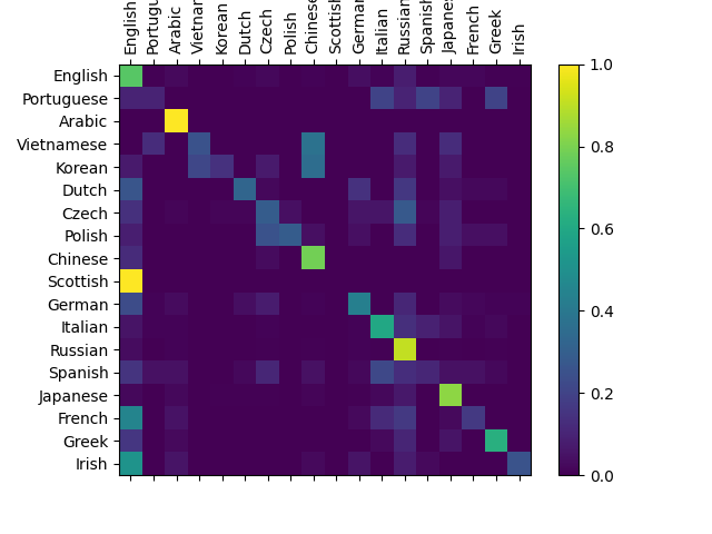
您可以在主對角線之外找出亮點，顯示它錯誤猜測的語言，例如將朝鮮語猜成中文，將義大利語猜成西班牙語。它在希臘語上表現非常好，而在英語上表現非常差（可能是因為與其它語言有重疊）。

練習¶

使用更大和/或形狀更好的網路獲得更好的結果
- 調整超引數以提高效能，例如更改 epoch 數、批次大小和學習率
- 嘗試 nn.LSTM 和 nn.GRU 層
- 修改層的大小，例如增加或減少隱藏節點的數量或新增額外的線性層
- 將這些 RNN 中的多個組合成一個更高層次的網路
嘗試使用不同的 line -> label 資料集，例如
- 任意單詞 -> 語言
- 名字 -> 性別
- 角色名 -> 作者
- 頁面標題 -> 部落格或 subreddit

指令碼總執行時間: ( 5 分 46.422 秒)

Gallery 由 Sphinx-Gallery 生成